
In this installment we focus on downloading, condensing, and uploading US Census TIGER data into PostGIS. The complete TIGER dataset is very large, and you should allocate enough time and space to download it all. As we go along, I will let you know how big a download you can expect and how much temporary space you will need to process them. I will be describing how to download, convert, and upload the files using my Ubuntu system. The instructions will be a bit different using Windows and you should consult your documentation as to how the utilities run there. I will be using the lftp program to download the files, tools from GDAL to do the processing, and shp2pgsql from PostGIS to upload the data.
The Census portion of the series covers a lot of information, so I am breaking it up into multiple parts to avoid having you fall asleep while reading a large document. This part focuses on the layout of the Census FTP site and what files are contained in each directory. I am also including pointers to the full Census TIGER documentation for a reading assignment. At the end, I will go over importing the Census state outlines so you at least have something to look at until next time.
I will be posting my own conversions of the TIGER dataset to this website. The Census puts data out at a county level. Personally, I prefer having the data at a state level and that is also how I import it into PostGIS. Plus, having it backed up at the state level is handy in case you accidentally blow away your data like I may have done just recently while preparing for this part of the series. So if you like, you could read along and then just download the condensed file from my site if you do not feel like running the conversions on your own.
At the time of this writing, the latest version of the data is 2013 and is available at http://www.census.gov/geo/maps-data/data/tiger-line.html. The Census makes the data available for download in Shapefile format inside of zip files for each county or national organizational unit. The first thing you should do is skim through the full technical documentation that is available in PDF format here. This document describes the data model used in the various file sets and what each field means inside the various files. It also describes what the files contain and their naming convention. This information is very useful if you intend to do more than just load data to look at a map.
We will be downloading the data from the main FTP site here. I will be using the lftp program under Linux to download the files, as it provides an easy way to download entire directories at a time. On Windows there are similar download managers you can use to accomplish the same task. When you ftp to the above site, you will see the following directory structure:
lftp ftp2.census.gov:/geo/tiger/TIGER2013> dir
-rw-rw-r-- 1 holla301 i-geo 228662 Aug 21 2013 2013-FolderNames-Defined.pdf
drwxrwsr-x 2 holla301 i-geo 143360 Aug 16 2013 ADDR
drwxrwsr-x 2 holla301 i-geo 167936 Aug 16 2013 ADDRFEAT
drwxrwsr-x 2 holla301 i-geo 143360 Aug 16 2013 ADDRFN
drwxrwsr-x 2 holla301 i-geo 4096 Aug 16 2013 AIANNH
drwxrwsr-x 2 holla301 i-geo 4096 Aug 16 2013 AITS
drwxrwsr-x 2 holla301 i-geo 4096 Aug 16 2013 ANRC
drwxrwsr-x 2 holla301 i-geo 4096 Aug 16 2013 AREALM
drwxrwsr-x 2 holla301 i-geo 167936 Aug 16 2013 AREAWATER
drwxrwsr-x 2 holla301 i-geo 4096 Aug 16 2013 BG
drwxrwsr-x 2 holla301 i-geo 4096 Aug 16 2013 CBSA
drwxrwsr-x 2 holla301 i-geo 4096 Aug 16 2013 CD
drwxrwsr-x 2 holla301 i-geo 4096 Aug 16 2013 CNECTA
drwxrwsr-x 2 holla301 i-geo 4096 Aug 16 2013 COAST
drwxrwsr-x 2 holla301 i-geo 4096 Aug 16 2013 CONCITY
drwxrwsr-x 2 holla301 i-geo 4096 Aug 16 2013 COUNTY
drwxrwsr-x 2 holla301 i-geo 4096 Aug 16 2013 COUSUB
drwxrwsr-x 2 holla301 i-geo 4096 Aug 16 2013 CSA
drwxrwsr-x 2 holla301 i-geo 135168 Aug 16 2013 EDGES
drwxrwsr-x 2 holla301 i-geo 4096 Aug 16 2013 ELSD
drwxrwsr-x 2 holla301 i-geo 4096 Aug 16 2013 ESTATE
drwxrwsr-x 2 holla301 i-geo 147456 Sep 13 12:24 FACES
drwxrwsr-x 2 holla301 i-geo 172032 Aug 16 2013 FACESAH
drwxrwsr-x 2 holla301 i-geo 4096 Aug 16 2013 FACESAL
drwxrwsr-x 2 holla301 i-geo 4096 Aug 16 2013 FACESMIL
drwxrwsr-x 2 holla301 i-geo 163840 Aug 16 2013 FEATNAMES
drwxrwsr-x 2 holla301 i-geo 180224 Aug 16 2013 LINEARWATER
drwxrwsr-x 2 holla301 i-geo 4096 Aug 16 2013 METDIV
drwxrwsr-x 2 holla301 i-geo 4096 Aug 16 2013 MIL
drwxrwsr-x 2 holla301 i-geo 4096 Aug 16 2013 NECTA
drwxrwsr-x 2 holla301 i-geo 4096 Aug 16 2013 NECTADIV
drwxrwsr-x 2 holla301 i-geo 126976 Aug 16 2013 OTHERID
drwxrwsr-x 2 holla301 i-geo 4096 Aug 16 2013 PLACE
drwxrwsr-x 2 holla301 i-geo 4096 Aug 16 2013 POINTLM
drwxrwsr-x 2 holla301 i-geo 4096 Aug 16 2013 PRIMARYROADS
drwxrwsr-x 2 holla301 i-geo 4096 Aug 16 2013 PRISECROADS
drwxrwsr-x 2 holla301 i-geo 4096 Aug 16 2013 PUMA
drwxrwsr-x 2 holla301 i-geo 4096 Aug 16 2013 RAILS
drwxrwsr-x 2 holla301 i-geo 155648 Aug 16 2013 ROADS
drwxrwsr-x 2 holla301 i-geo 4096 Aug 16 2013 SCSD
drwxrwsr-x 2 holla301 i-geo 4096 Aug 16 2013 SLDL
drwxrwsr-x 2 holla301 i-geo 4096 Aug 16 2013 SLDU
drwxrwsr-x 2 holla301 i-geo 4096 Aug 16 2013 STATE
drwxrwsr-x 2 holla301 i-geo 4096 Aug 16 2013 SUBMCD
drwxrwsr-x 2 holla301 i-geo 4096 Aug 16 2013 TABBLOCK
drwxrwsr-x 2 holla301 i-geo 4096 Aug 16 2013 TBG
drwxrwsr-x 2 holla301 i-geo 4096 Aug 16 2013 TRACT
drwxrwsr-x 2 holla301 i-geo 4096 Aug 16 2013 TTRACT
drwxrwsr-x 2 holla301 i-geo 4096 Aug 16 2013 UAC
drwxrwsr-x 2 holla301 i-geo 4096 Aug 16 2013 UNSD
drwxrwsr-x 2 holla301 i-geo 4096 Aug 16 2013 ZCTA5
As to what these directories contain, here is a summary taken from the TIGER documentation. As we load each file type, I will cover what the files contain in more detail.
- ADDR – Address Range Relationship File. These files contain DBF files that contain address information for each edge in the dataset. For each edge, it lists the from- and to- house numbers, which side of the road they are on, the ZIP, and ZIP+4 codes.
- ADDRFEAT – Address Range Feature File. These files are Shapefiles that contain information similar to the above and other metadata such as street names.
- ADDRFN – Address Range-Feature Name Relationship File. Each file maps the relationship between address range and linear feature identifiers.
- AIANNH – American Indian / Alaska Native / Native Hawaiian Areas. This national-level file contains federally-recognized American Indian reservations and off-reservation trust land areas, state-recognized reservations, and Hawaiian home land areas for which the Census publishes data.
- AITSN – American Indian Tribal Subdivision National. Another national-level file that contains legally defined administrative subdivisions of federally-recognized American Indian reservations, off-reservation trust lands, or Oklahoma tribal statistical areas.
- ANRC – Alaska Native Regional Corporation. These are areas that define corporate entities established to conduct both business and nonprofit affairs of the Alaska Natives pursuant to the Alaska Native Claims Settlement Act of 1972.
- AREALM – Area Landmarks. These files contain area landmarks that the Census records for locating special features and to help enumerators during field operations (parks, schools, etc).
- AREAWATER – Area Water. These contain polygonal area definitions of water (or hydrographic) features such as lakes, ponds, and rivers.
- BG – Block Groups. These are Census-specific clusters of blocks that have the same first digit of their four-digit identifying numbers within a Census Tract.
- CBSA – Metropolitan Statistical Area / Micropolitan Statistical Area. These Shapefiles contain the 2013 county and equivalent entities and contain fields with codes for combined, metropolitan, or micropolitan statistical areas and metropolitan divisions.
- CD – Congressional District. These are area definitions of the 113th Congressional Districts.
- CNECTA – Combined New England City and Town Area. These files contain the Office of Management and Budget (OMB)-defined alternative county subdivision-based definitions of statistical areas known as New England city and town areas.
- COASTLINE – US Coastlines. This is a new addition that is a national-level file of linear coastline features.
- CONCITY – Consolidated Cities. These are defined as units of local governments for which the functions of the incorporated place and its county or minor civil division have merged.
- COUNTY – US Counties. This is a national-level file containing the definitions for counties within the US and its territories.
- COUSUB – County Subdivision. These are statistical subdivisions of boroughs, city nad boroughs, municipalities, and census areas.
- CSA – Combined Statistical Area. These are groups of two or more areas that have significant employment interchanges.
- EDGES – All linear edges in the dataset. These data contain every edge that the Census has recorded, be it road, rail, or water features.
- ELSD – Elementary School District. These are area definitions that define locality-recognized elementary school districts.
- ESTATE – Estates. These are subdivisions of the three major islands in the United States Virgin Islands that have legally defined boundaries and are generally smaller in area than the Census subdistricts.
- FACES – Topological Faces (Polygons With All Geocodes). Faces are areal objects that are bounded by one or more edges and are topological primitives. A face is not internally subdivided by edges into smaller polygons but may completely surround other faces (such as islands).
- FACESAH – Topological Faces-Area Hydrography Relationship File. These are face areas that contain a water feature relationship.
- FACESAL – Topological Faces-Area Landmark Relationship File. These are face areas that contain a landmark feature relationship.
- FACESMIL – Topological Faces-Military Installation Relationship File. These are face areas that contain a military feature relationship.
- FEATNAMES – Feature Names Relationship File. These files contain a record for each feature name-edge combination and includes the feature name attributes. This file may contain alternative names for linear features.
- LINEARWATER – Linear Water. This file contains linear features where the edge represents a water feature.
- METDIV – Metropolitan Division. These files represent metropolitan statistical areas containing a single core with a population of at least 2.5 million people and is subdivided to form smaller groupings of counties or equivalent entities.
- MIL – Military Installations. This is a national-level file denoting US military installations.
- NECTA – New England City and Town Area. These files contain the areas covered by the OMB for Combined New England city and town areas.
- NECTADIV – New England City and Town Area Division. These areas are created when a NECTA containing a single core with a population of at least 2.5 million is to form smaller groupings of cities and towns.
- OTHERID – Other Identifiers. This file contains external identifier codes and individual county identifiers between the permanent edge identifier attribute in the EDGES file and the identifier listed here.
- PLACE – Places. These files contain geography and attributes at the state level of both incorporated places and census designated places.
- POINTLM – Point Landmarks. These are point features that are used to locate special features and to help enumerators during field operations. They contain points that identify areas such as airports, parks, and schools.
- PRIMARYROADS – Primary Roads. These are defined as generally divided, limited-access highways within the Federal interstate highway system or under state management.
- PRISECROADS – Primary and Secondary Roads. These files contain the primary roads and main arteries that are usually in a US, state, or county highway system with one or more lanes of traffic in each direction.
- PUMA – Public Use Microdata Area. These are decennial census areas that have been definied for the tabulation and dissemination of public use microdata sample American Community Survey data.
- RAILS – Railroads. These are linear edges that denote railroads at the national level.
- ROADS – All roads. These files contain all roads (major or minor) in the US and its territories.
- SCSD – Secondary School District. These are secondary school districts that are typically defined as between elementary school and college.
- SLDL – State Legislative District – Lower Chamber. These areas denote state legislative districts that are equivalent to a house chamber.
- SLDU – State Legislative District – Upper Chamber. These areas denote state legislative districts that are equivalent to a senate chamber.
- STATE – State and Equivalent. These files contain the outlines of each state and territory in the US.
- SUBBARRIO – SubMinor Civil Division (Subbarrios in Puerto Rico). These areas are legally defined divisions or minor civil divisions in Puerto Rico.
- TABBLOCK – Tabulation (Census) Block. These areas are definied by the Census as statistical areas bounded on all sides by visible features, such as streets, roads, streams, railroad tracks, and by non-visible boundaries such as city, town, township, and county limits.
- TBG – Tribal Block Group. These areas are clusters of blocks within the same tribal census tract.
- TRACT – Census Tract. These areas are small, relatively permanent statistical subdivisions of a county or equivalent entity and are reviewed and updated by local participants prior to each decennial census as part of the Census Bureau’s Participant Statistical Areas Program.
- TTRACT – Tribal Census Tract. These are relatively small statistical subdivisions of an American Indian reservation and/or off-reservation trust land and were defined by federally recognized tribal government officials working with the Census.
- UAC – Urban Area/Urban Cluster. These are clusters consisting of densely developed territory that has between 2,500 and 50,000 people.
- UNSD – Unified School District. These are pseudo-secondary school districts that represent regular unified school districts in areas where the unified school district share final responsibility with the elementary district.
- ZCTA5 – 5-Digit ZIP Code Tabulation Area. These are approximate area representations of US Postal Service five digit ZIP code service areas that the Census creates using whole blocks to present statistical data from censuses and surveys.
Census State Outlines
We first need a database to hold all of the Census data. If you created a geospatial database template from earlier in this series, open a shell prompt and type:
createdb -T gistemplate Census_2013
Now that we have gone through all of that, the first dataset we will upload is only 8.3 megabytes in size. From the shell prompt, run:
mkdir census
cd census
Again from the shell prompt, run
lftp ftp://ftp2.census.gov/geo/tiger/TIGER2013.
You should see something similar to the below:
lftp ftp://ftp2.census.gov/geo/tiger/TIGER2013
cd ok, cwd=/geo/tiger/TIGER2013
lftp ftp2.census.gov:/geo/tiger/TIGER2013>
You can then type cls to get a shortened listing of the directories I just described. From inside the client, type:
mirror STATE/
lftp will download the file and once done you will see something like this:
lftp ftp2.census.gov:/geo/tiger/TIGER2013> mirror STATE/
Total: 1 directory, 1 file, 0 symlinks
New: 1 file, 0 symlinks
8599274 bytes transferred in 17 seconds (500.2K/s)
lftp ftp2.census.gov:/geo/tiger/TIGER2013>
You can now type quit and hit enter or type Control-D to exit lftp. Change into the directory STATE and you will see this file:
[bmaddox@girls STATE]$ ls -l
total 8400
-rwxrw-r-x 1 bmaddox bmaddox 8599274 Aug 16 2013 tl_2013_us_state.zip
[bmaddox@girls STATE]$
This follows the Census naming convention of:
- tl = TIGER/Line
- 2013 = the version of the files
- us = parent geography entity ID code of the geographic extent, in this case US being the entire country.
- State = layer tag for the dataset
- zip = the file extension
Run unzip tl_2013_us_state.zip and you will then find these files in the STATE directory:
[bmaddox@girls STATE]$ unzip tl_2013_us_state.zip
Archive: tl_2013_us_state.zip
inflating: tl_2013_us_state.dbf
inflating: tl_2013_us_state.prj
inflating: tl_2013_us_state.shp
inflating: tl_2013_us_state.shp.xml
inflating: tl_2013_us_state.shx
[bmaddox@girls STATE]$ ls
tl_2013_us_state.dbf tl_2013_us_state.shp tl_2013_us_state.shx
tl_2013_us_state.prj tl_2013_us_state.shp.xml tl_2013_us_state.zip
[bmaddox@girls STATE]
These files make up the ESRI Shapefile format. For a more complete explanation of what each file is, consult the links to the format that I have posted previously in this series.
To upload the files to PostGIS with the proper geographic coordinates, we need to know the EPSG code of the data that defines its projection. All Census TIGER data uses the EPSG code 4269 which denotes the NAD83 datum.
From this directory, run the following command to create a table with the state outlines and your output should look similar to the below:
[bmaddox@girls STATE]$ shp2pgsql -s 4269 -c -D -I tl_2013_us_state.shp State_Outlines | psql -d Census_2013
Shapefile type: Polygon
Postgis type: MULTIPOLYGON[2]
SET
SET
BEGIN
NOTICE: CREATE TABLE will create implicit sequence "state_outlines_gid_seq" for serial column "state_outlines.gid"
CREATE TABLE
NOTICE: ALTER TABLE / ADD PRIMARY KEY will create implicit index "state_outlines_pkey" for table "state_outlines"
ALTER TABLE
addgeometrycolumn
----------------------------------------------------------------
public.state_outlines.geom SRID:4269 TYPE:MULTIPOLYGON DIMS:2
(1 row)

CREATE INDEX
COMMIT
[bmaddox@girls STATE]$
The options to the command line are:
- -s = specify the EPSG code
- -c = create a table
- -D = use postgresql dump format (speeds things up basically)
- -I = create a spatial index column. This column contains the coordinates of the line segments so a GIS can determine where they are
- State_Outlines = the table name to create
- | psql -d Census_2013 = takes the output from the shp2pgsql command and pipes it to the psql command using the Census_2013 database.
To view the data, run QGIS Desktop. As I discussed earlier in the series, open the load from PostGIS dialog and create an entry called Census_2013 with the hostname, database, user, and password for your specific setup. Once that is done, click Connect and expand the entries under the public schema and you should see something like this:

Census 2013 Table with State Outlines
Click the state_outlines layer and then the Add button. After a second or two you should see this:
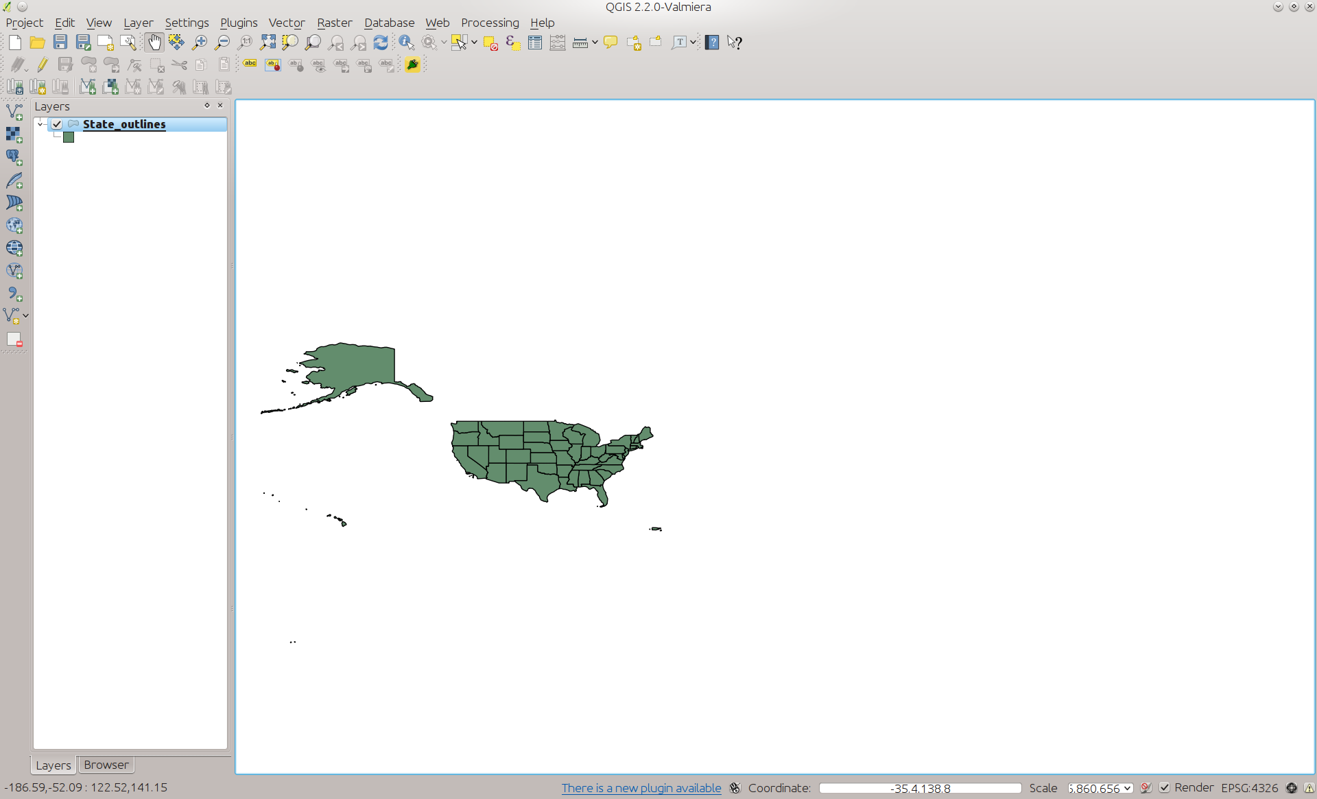
State Outlines table in QGIS
And that is it. Fairly easy, eh? You have just successfully learned a bit about the Census TIGER dataset, put data into PostGIS, and viewed it inside QGIS. You can right click on the layer in QGIS to view the attribute table to see what kind of data is stored for each state.
Next time, we will continue working through TIGER data to create your first large-scale geospatial database.