All of the previous parts of this series have talked about the challenges in training a CNN to detect geological features in LiDAR. This time I will talk about actually running the CNN against the test area and my thoughts on how it went.
Detection
I was surprised at how small the actual network was. The xCeption model that I used ended up only being around 84 megabytes. Admittedly this was only three classes and not a lot of samples, but I had expected it to be larger.
Next, the test image was a 32-bit single band LiDAR GeoTIFF that was around 350 gigabytes. This might not sound like much, but when you are scanning it for features, believe me it is quite large.
First off, due to the size of the image, and that I had to use a sliding window scan, I knew that the processing time would be long to run detections. I did some quick tests on subsections and realized that I would have to break up the image and run detection in chunks. This was before I had put a water cooler on my Tesla P40, and since I wanted to sleep at night, just letting it run to completion was out of the question. Sleep was not the only concern I had. I live south of the capital of the world’s last superpower, yet at the time we lost power any time it got windy or rained. The small chunks meant that if I lost power, I would not lose everything and could just restart it on the interrupted part.
I decided to break the image up into an 8×8 grid. This provided a size where each tile could be processed in two to three hours. I also had to generate strips that covered the edges of the tiles to try to capture features that might span two tiles. I had no idea how small spatially a feature could be, so I picked a 200×200 minimum pixel size for the sliding window algorithm. This still meant that each tile would have several thousand potential areas to run detections against. In the end it took several weeks worth of processing to finish up the entire dataset (keeping in mind that I did not run things at night since it would be hard to sleep with a jet engine next to you).
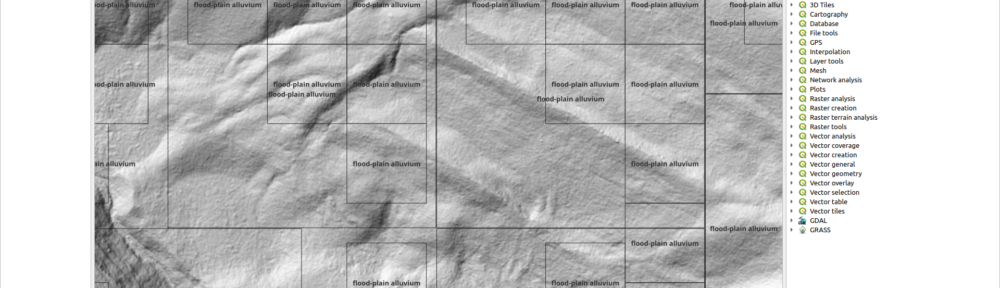
How well did it work? Well, that’s the interesting part. I’m not a geomorphologist so I had to rely on the client to examine it. But here’s an example of how it looks via QGIS:

As you can see, it tends to see a lot of areas as floodplain alluvium. After consulting with the subject matter experts, there are a few things that stand out.
- The larger areas are not as useful as the smaller ones. As I had no idea of a useful scale, I did not have any limitations to the size of the bounding areas to check. However, it appears the smaller boxes actually do follow alluvium patterns. The output detections need to be filtered to only keep the smaller areas.
- It might be possible to run a clustering algorithm against the smaller areas to better come up with larger areas that are correctly in the class.
Closing thoughts and future work
While mostly successful, as I have had time to look back, I think there are different or better ways to approach this problem.
The first is to train on the actual LiDAR points versus a rasterization of them. Instead of going all the way to rasterization, I think keeping the points that represent ground level as inputs to training might be a better way to go. This way I could alleviate the issues with computer vision libraries and potentially have a simpler workflow. I am curious if geographic features might be easier for a neural network to detect if given the raw points versus a converted raster layer.
If I stay with a rasterized version, I think if I did it again I would try one of the YOLO-class models. These models are state-of-the-art and I think may work better in scanning large areas for smaller scale features as it does its own segmentation and detection. The only downside to this is I am not entirely sure YOLO’s segmentation would identify areas better than selective search due to the type of input data.
I think it would also be useful to revisit some of the computer vision algorithms. I believe selective search could be extended to work with higher numbers of bits per sample. Some of the other related algorithms could likely be extended. This would help in general with remotely sensed data as it usually contains higher numbers of bits per sample.
While there are a lot of segmentation models out there, I am curious how well any of them would work with this type of data. Many of them have the same limitations as OpenCV does and cannot handle 32-bits per sample imagery. These algorithms typically images where objects “stand out” against the background. LiDAR in this case is much different than the types of sample data that such images were trained on. For example, here is a sample of OpenCV’s selective search run against a small section of the test data. The code of course has to convert the data to 8-bits/sample and convert it to a RGB image before running. Note that this was around 300 meg in size and took over an hour to run on my 16 core Ryzen CPU.

You can see that selective search seems to have trouble with this type of LiDAR as there are not anything such as house lots that could be detected. The detections are a bit all over the place.
Well that’s it for now. I think my next post will be about another thing I’ve been messing with: applying image saliency algorithms to LiDAR just to see if they’d pull anything out.