I came across an old backup set the other day and found a copy of the CVS -> Subversion repository I kept that included a lot of code that I wrote, inherited, or maintained. The code is at least ten years old now so likely not of use to anyone. I mainly did it to preserve the source for historical reasons. If anyone is interested, you can find it at https://github.com/briangmaddox.
Category Archives: Uncategorized
Census 2015 State/National Data Remix Done
Yes, just in time for 2016… I’ve finished uploading and changed the links for the 2015 Census Tiger data converted to state or national datasets from the county files. I’ve also stopped posting the single-file entries as there is not really a need to do that. Hop over to https://brian.digitalmaddox.com/blog/?page_id=202 if you’re interested.
No, Using Interfaces (or Abstractions) Alone Does NOT Mean You’re “Object Oriented”
Since I’ve been dealing with a lot of Java and now C# code over the past few years, I’ve noticed one thing: Java and C# programmers love interface classes. In fact, it seems that most Java and C# programmers think that they cannot have a concrete class that does not inherit from some interface. I was curious about this in a lot of the C# code I’ve had to deal with so I asked why. The answer I got was “that way we are using abstractions and encapsulating things.”
Wrong. Just, wrong.
“Why not smart guy?” you might ask. First off, let’s look at some definitions. An interface is used to define a set of functionality that derived classes must implement. Interfaces can only contain method and constant declarations, not definitions. An abstraction reduces and factors out details so that the developer can focus on only a few concepts at a time. It is similar to an interface, but instead of only containing declarations, it can contain partial definitions while forcing derived classes to re-implement certain functionality.
With these definitions, we see that an interface is just a language construct. It really just specifies a required syntax. In some languages, they are not even classes. What went wrong? Well, historically, it appears that people got the wrong idea that an interface splits contracts from implementations, which is a good thing in object-oriented programming because it encapsulates functionality. An implementation does not do this, IT CAN’T. Remember, an interface simply specifies what functions must be present and what their returns are. It does not enforce how computations should be done. Consider the following interface pseudo code that defines an imaginary List with a count variable that specifies how many elements are in the list:
interface MyList
{
public void AddItem(T item);
public int GetNumItems();
}
So, where does the above enforce a contract that each added item will increment an internal counter? How does it FORCE me as a programmer to increment an internal counter? It doesn’t; it can’t. Since an interface is purely an empty shell, I as a user am free to do as I like as long as I just follow the interface definition. If I don’t want to increment an internal counter, I don’t have to do so. This does not really fulfill the object oriented dependency inversion principle (DIP), which states (as quoted by Wikipedia):
A. High-level modules should not depend on low-level modules. Both should depend on abstractions. B. Abstractions should not depend on details. Details should depend on abstractions
In common speak, this basically means that we can focus on high-level design and issues by ignoring the low-level details. We use abstractions to encapsulate functionality so that we are guaranteed that the low-level details are taken care of for us. Consider the following pseudo code abstract List class:
abstract class MyList
{
public void AddItem(T item)
{
AbstractedAdd(item);
this.internalcounter++;
}
public int GetNumItems()
{
return this.internalcounter;
}
abstract private void AbstractedAdd(T item);
}
With the abstract class, we actually have a contract now that fulfills the DIP. As an abstraction can contain a partial definition, we have a defined AddItem() function that calls an abstract internal function but also increments the internal counter. While it is a loose guarantee, we are guaranteed that the internal counter is incremented every time AddItem() is called. We now do not have to worry that the abstraction will take care of the item counter for us.
What appears to have happened over the years is that student programmers heard about things like the DIP and warped it to think it means that every class must have an interface (when they mean abstraction), whether or not the class is designed to be used only once. This I think can be attributed to teachers not doing a good job at differentiating interfaces from abstractions and not really teaching what encapsulation means. Thinking like this also led to the second problem.
Secondly, a lot of people did not get the message that “all software should be designed to be reusable” got discredited after the 1990’s when it turned out that this philosophy needlessly complicates code. Trying to design code like this ends up with a huge Frankenstein’s monster that is hopelessly complex, prone to errors, and really does not face reality that being a Jack of all trades means you’re a master of none. This created a somewhat tongue-in-cheek object oriented principle called the Reused Abstraction Principle (RAP) that says “having only one implementation of a given interface is code smell.” We refactor code to pull out duplicate functionality because it helps to keep the code base small. It improves reliability because having a single implementation of potentially duplicated code means we don’t have several duplicate implementations that may differ in how they are done.
However, this does not mean that code HAS to have duplicated functionality “just because.” If your problem domain only has one instance of a use case, it really is OK to just have a single concrete class that implements this. Focus on a good design that encapsulates the functionality of your problem domain, not worrying that every piece of functionality must be reusable. Later on, if you problem domain is expanded and you end up with duplicate functionality, refactor it and then have an interface or abstract class. Needless use of interfaces and abstractions just doubles the number of classes in your code base, and in most languages abstractions will have a performance penalty due to issues like virtual table lookups. Simple use of interfaces and abstractions does not make you a cool kid rock-star disciple of the Gang of Four.
The Day After
Updating the Merged TIGER Files to the 2014 Dataset
Hey all, I am finally in the process of updating my merged state- and national-level TIGER files to the 2014 data that they have put out. You can find them at my GIS Data Page. Note that Roads are not uploaded yet but I already updated the links on the download page so you will get 404 errors until I get them uploaded. I cannot promise it will be tonight since I have to sleep sometime 😉 If you find any 404s on the others, let me know in case I missed a link.
As usual, these are my own value added files that I am publishing in case some people find them useful. If you use these and your business fails, your wife leaves you, your dog dies, and you write a country music song about it, not my fault.
More Fun with Old Maps
I’ll admit it, I really like old maps. I especially like old topographic maps. I think it started when I used to work for the US Geological Survey. To me, it’s interesting to see how things change over time. From my old urban grown prediction days, I like to see where and when populations change.
Since the USGS put out their Historical Topographic Map Collection (HTMC), I’ve been playing with the maps off and on for about a year now. I finally decided to start merging available maps of the same scale and vintage to study and possibly do feature extraction down the road. I’ll be placing them for download here in case anyone is interested as I process them.
I thought I’d share how I put them together in case anyone else is interested. The first step is to go to the USGS website and pick the files you want to use. The files there are available in GeoPDF format. First thing you need to understand is that you may not find a map covering your area of interest at your scale of interest and vintage. Not everything managed to survive to the current day. For example, I made a merged 125K map of Virginia and most of southern VA is missing at that resolution.
Once I download the GeoPDFs I want to work on, I use a modified version of the geopdf2gtiff.pl script from the Xastir project. The link to my modifications can be found here. I use LZW compression for my GeoTIFFs as it’s lossless and keeps the quality from the GeoPDFs. It is a Perl script and requires that you have GDAL and the GDAL API installed. What it does is calculate the neat-lines of the GeoPDF and then clips it to the neat-line while converting it to a GeoTIFF. Running it as as simple as:
geopdf2gtiff.pl inputfile.pdf
Once you have all of your GeoPDF files download and converted, the next step is to merge them. The fastest way I’ve found to merge involves using gdalbuildvrt and gdal_translate, also from GDAL. The first step is to create a virtual dataset of all of your files by running something like:
gdalbuildvrt -resolution highest -a_srs EPSG:4326 merged.vrt parts/*.tif
The options I chose here are to pick the highest pixel resolution (-resolution) based on the input files. For this case the resolutions should be the same, but this way I don’t have to go through and verify that. Next I change the projection of the output file to WGS84 (-a_srs). Next is the file name of the virtual dataset and then the input files.
Now that the virtual dataset is done, it’s time to actually merge all of the files together. The virtual dataset contains the calculated bounding box that will contain all of the input files. Now we use gdal_translate to actually create the merged GeoTIFF file:
gdal_translate -of GTiff -co COMPRESS=LZW -co PREDICTOR=2 merged.vrt ~/merged.tif
Here again I use LZW compression to losslessly compress the output data. Note that gdal_translate will automatically add an Alpha channel as Band 4 in the image to denote areas that had no input data. That’s why we do NOT add the -addalpha flag to gdalbuildvrt. For performance tips, I’d suggest keeping the source data and output file on separate drives unless you’re running something like a solid state drive. To give you an idea of the output file sizes, Virginia merged (which did have a lot of areas missing), was around 500 megabytes.
Next you’ll need a Shapefile to use as a cut file to clip the data. Since I have the Census Tiger 2013 data in a local PostGIS database (see previous posts to this blog), I used QGIS to select just the VA state outline and then saved it as a Shapefile.
Finally, we will use gdalwarp to clip the merged GeoTIFF against the state outline to produce the clipped GeoTIFF that is just the state itself. This operation can take a bit of time depending on how powerful a machine you’re running it on. The command you will use is similar to this:
gdalwarp --config GDAL_CACHEMAX 1024 -wm 1024 -cutline va_outline.shp -crop_to_cutline -multi -t_srs EPSG:4326 -co COMPRESS=LZW -co PREDICTOR=2 -co BIGTIFF=YES -co TILED=YES ~/merged.tif clipped.tif
Some of the command line parameters I used are optional, I just tend to leave them in since I do a lot of copying and pasting 😉 First we tell GDAL to increase the size of its caches using the –config GDAL_CACHEMAX and -wm options. Next we specify the file to clip against with the -cutline and -crop_to_cutline options. The -multi option tells GDAL to process using multiple threads. I again specify the output projection and the LZW compression parameters. Here I also specify the BIGTIFF option just in case the output file goes over four gigabytes. Finally, I tell gdalwarp to tile the output TIFF so it will load faster in a GIS by separating it into tiles.
The output will look something like the below figure. I’ll start posting files as I get time. Hope everyone is having a great holiday!
Keeping up with the Botnets Round 2
I’ve been keeping up with tracking how many botnets are out there scanning WordPress blogs. I’ve eventually resorted to blocking huge chunks of the Internet via .htaccess files. So far it’s been quite effective in limiting the number of botnet login attempts.
If anyone is interested, I’ve put the limit portion of my .htaccess file here. Feel free to use it and customize for your needs.
Some Website Changes thanks to Botnets
Lately I’ve been getting tons and tons of login attempts from what appear to be botnets. Since I’m getting tired of banning the IPs individually, I’m temporary taking to banning entire countries and ISP’s from hitting my blog. If you’re in that group, sorry guys. Take it up with your ISP.
Here are some stats I’ve been gathering.
IP Addresses Grouped by ISPs
| 217.16.9.99 | ab connect |
| 174.142.104.207 | angmalta.net ltd. |
| 80.97.64.148 | astral telecom sa |
| 79.182.60.204 | bezeq international-ltd |
| 112.196.2.36 | chandigarh |
| 60.12.119.200 | china unicom zhejiang province network |
| 14.147.73.105 | chinanet guangdong province network |
| 216.222.148.52 | chl |
| 119.82.71.107 | citycom networks pvt ltd |
| 69.64.65.10 | codero |
| 203.195.184.151 | comsenz technology ltd |
| 88.190.45.37 | dedibox sas |
| 177.70.21.29 | desenvolve solucoes de internet ltda |
| 176.9.195.105 | desokey mohamed hassan centerarabs |
| 66.147.235.81 | dotblock.com |
| 166.63.127.244 | ecommerce corporation |
| 122.213.243.131 | erfahren co. ltd. |
| 198.50.112.114 | faan international |
| 50.7.139.53 | fdcservers.net |
| 87.255.57.169 | fiberring b.v. |
| 42.62.24.250 | forest eternal communication tech. co.ltd |
| 216.98.196.14 | forethought.net |
| 42.112.19.220 | fpt telecom company |
| 117.18.73.66 | gigahost limited |
| 67.215.7.226 | globotech communications |
| 188.121.62.249 | go daddy netherlands b.v. |
| 118.139.162.178 | godaddy.com |
| 50.62.41.168 | godaddy.com llc |
| 50.63.57.211 | godaddy.com llc |
| 50.63.85.76 | godaddy.com llc |
| 50.63.130.155 | godaddy.com llc |
| 50.63.141.164 | godaddy.com llc |
| 97.74.127.145 | godaddy.com llc |
| 184.168.109.23 | godaddy.com llc |
| 184.168.112.26 | godaddy.com llc |
| 188.64.170.221 | h1 llc |
| 188.64.171.181 | h1 llc |
| 5.9.121.109 | hetzner online ag |
| 46.4.20.133 | hetzner online ag |
| 221.132.33.175 | ho chi minh city post and telecom company |
| 69.28.199.40 | host papa inc. |
| 184.171.240.27 | hostdime.com inc |
| 69.85.84.194 | hostigation |
| 82.145.45.104 | iomart hosting limited |
| 182.18.175.246 | ip pool for ctrls |
| 212.112.232.106 | ipx server gmbh |
| 195.93.180.34 | itsoft ltd |
| 64.15.138.14 | iweb dedicated cl |
| 46.165.206.78 | leaseweb germany gmbh |
| 64.31.25.60 | limestone networks inc |
| 173.255.217.143 | linode |
| 106.187.47.170 | linode llc |
| 188.191.53.8 | lubos hutar |
| 64.202.240.136 | mainstream consulting group inc |
| 64.207.147.191 | media temple inc |
| 70.32.107.181 | media temple inc |
| 205.186.142.240 | media temple inc. |
| 216.70.68.242 | media temple inc. |
| 89.200.138.207 | memset ltd |
| 85.112.29.210 | nap de las americas-madrid s.a. |
| 212.82.217.9 | neocom-service isp |
| 69.163.164.235 | new dream network llc |
| 85.204.118.142 | nixway srl |
| 41.190.76.5 | onesolutions |
| 125.253.118.46 | online data services jsc |
| 212.83.164.81 | online s.a.s. |
| 88.151.245.66 | openminds bvba |
| 142.4.208.97 | ovh hosting inc |
| 5.39.106.19 | ovh sas |
| 5.135.165.206 | ovh sas |
| 5.135.188.80 | ovh sas |
| 37.59.29.48 | ovh sas |
| 37.59.35.4 | ovh sas |
| 37.187.67.49 | ovh sas |
| 46.105.105.58 | ovh sas |
| 91.121.86.86 | ovh sas |
| 188.165.202.118 | ovh sas |
| 162.211.82.114 | privatesystems networks |
| 83.96.132.85 | proserve b.v. |
| 210.210.178.20 | pt. cyberindo aditama |
| 112.78.44.28 | pt. des teknologi informasi |
| 31.210.117.13 | radore veri merkezi hizmetleri a.s. |
| 82.79.27.158 | rcs & rds business |
| 185.9.157.31 | salay telekomunikasyon ticaret limited sirketi |
| 89.47.253.2 | sc eurosistem srl |
| 46.102.232.243 | sc webfactor srl |
| 64.34.173.227 | serverbeach |
| 31.24.36.35 | serverspace limited |
| 69.175.111.218 | singlehop inc |
| 108.178.57.146 | singlehop inc |
| 173.236.21.58 | singlehop inc |
| 91.189.219.107 | skyware sp. z o.o. |
| 190.107.177.102 | soc. comercial wirenet chile ltda. |
| 108.59.252.133 | softcom america inc. |
| 108.59.254.26 | softcom america inc. |
| 50.97.138.111 | softlayer technologies inc |
| 85.214.27.40 | strato ag |
| 85.214.64.100 | strato ag |
| 85.214.153.62 | strato ag |
| 46.235.9.199 | teknik data internet teknolojileri san.tic.ltd. sti |
| 37.205.32.122 | tolvu- og rafeindapjonusta sudurlands ehf |
| 95.0.26.85 | turk telekomunikasyon anonim sirketi |
| 123.30.208.178 | vietnam data communication company |
| 222.255.29.39 | vietnam data communication company |
| 37.122.210.63 | webfusion internet solutions |
| 91.109.3.166 | webfusion internet solutions |
| 212.48.67.110 | webfusion internet solutions |
| 192.254.202.144 | websitewelcome.com |
| 62.212.130.150 | xenosite b.v. |
As you can see, I get a bunch from Godaddy and French ISP Ovh. I’ve also banned Godaddy IP’s, Ovh, and Media Temple. I’ll be adding others once I find all of their allocated net ranges.
For reference, here’s a copy of my current list along with attempts:
| IPs | Attempts |
| 106.187.47.170 | 34 |
| 108.59.252.133 | 26 |
| 118.139.162.178 | 20 |
| 122.213.243.131 | 1 |
| 123.30.208.178 | 3 |
| 142.4.208.97 | 12 |
| 162.211.82.114 | 1 |
| 166.63.127.244 | 63 |
| 174.142.104.207 | 1 |
| 182.18.175.246 | 8 |
| 184.168.109.23 | 16 |
| 184.168.112.26 | 23 |
| 185.9.157.31 | 26 |
| 188.121.62.249 | 43 |
| 188.165.202.118 | 12 |
| 188.191.53.8 | 3 |
| 188.64.170.221 | 232 |
| 188.64.171.181 | 5 |
| 190.107.177.102 | 13 |
| 195.93.180.34 | 34 |
| 198.50.112.114 | 52 |
| 203.195.184.151 | 53 |
| 205.186.142.240 | 43 |
| 210.210.178.20 | 87 |
| 212.112.232.106 | 1 |
| 212.48.67.110 | 4 |
| 216.222.148.52 | 1 |
| 216.70.68.242 | 12 |
| 216.98.196.14 | 1 |
| 221.132.33.175 | 1 |
| 222.255.29.39 | 18 |
| 31.210.117.13 | 1 |
| 37.122.210.63 | 6 |
| 37.205.32.122 | 33 |
| 37.59.29.48 | 81 |
| 37.59.35.4 | 27 |
| 41.190.76.5 | 14 |
| 42.62.24.250 | 6 |
| 46.102.232.243 | 9 |
| 46.105.105.58 | 28 |
| 46.165.206.78 | 112 |
| 46.235.9.199 | 18 |
| 46.4.20.133 | 3 |
| 5.135.165.206 | 180 |
| 5.135.188.80 | 6 |
| 5.39.106.19 | 46 |
| 5.9.121.109 | 61 |
| 50.62.41.168 | 7 |
| 50.63.130.155 | 19 |
| 50.63.141.164 | 13 |
| 50.97.138.111 | 2 |
| 60.12.119.200 | 32 |
| 62.212.130.150 | 24 |
| 64.202.240.136 | 48 |
| 64.207.147.191 | 13 |
| 64.31.25.60 | 83 |
| 64.34.173.227 | 244 |
| 66.147.235.81 | 39 |
| 67.215.7.226 | 19 |
| 69.175.111.218 | 1 |
| 69.64.65.10 | 3 |
| 70.32.107.181 | 1 |
| 80.97.64.148 | 4 |
| 82.145.45.104 | 8 |
| 83.96.132.85 | 46 |
| 85.112.29.210 | 58 |
| 85.204.118.142 | 1 |
| 85.214.153.62 | 4 |
| 85.214.64.100 | 27 |
| 87.255.57.169 | 175 |
| 88.190.45.37 | 1 |
| 89.200.138.207 | 1 |
| 89.47.253.2 | 58 |
| 91.109.3.166 | 2 |
| 95.0.26.85 | 20 |
| 97.74.127.145 | 36 |
| Total Attempts: | 2469 |
Guess I should be flattered that I’m getting all of this “attention” 🙂
The Lost Research Paper
Towards the end of my tenure at the US Geological Survey, I was the project manager and principal investigator of Restoration of Data from Lossy Compression. The goal of the project was to find ways to restore fine detail that was lost during lossy compression processes such as JPEG. I had submitted an Open File report through the review process, but left the USGS in 2006 before the paper had completed review. As I had left, it basically fell through the cracks and was never officially published.
I had forgotten about it until recently when I was updating my resume. So, without further ado, I have put the paper here. I took out the USGS logo and what not since it was never officially published by them. So for a flashback into what I was doing in 2006, have fun reading it 🙂
Using Free Geospatial Tools and Data Part 3: Understanding Geospatial Data
Before going into what tools and data are available, I feel a quick introduction to geospatial data is in order. I’m going to gloss over some things and greatly oversimplify others. If you want to know more, I would suggest checking out books such as Map Projections: A Working Manual by Snyder or some excellent tutorials on map projections and GIS that can be found via your favorite web search engine.
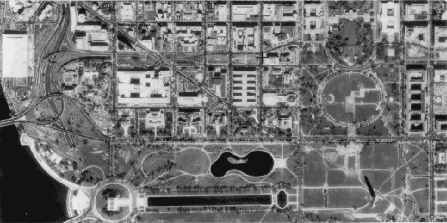
To begin, there are two main types of geospatial data available: raster and vector. Raster data are usually things such as aerial or satellite photographs, scanned paper maps, and so on. Vector data are mathematical vectors that describe items such as lines for roads, polygons for areas like parks, and others. As is, aerial photographs or vectors do not fully describe the Earth’s surface. They do not represent a one to one correlation between a point on the map and a location on the ground. They have to be run through a process called georectification to mathematically translate them to a coordinate system known as a map projection.
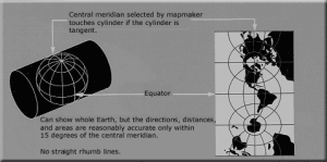
Map projections are mathematical descriptions of the surface of the Earth. As most of you (hopefully) know, the Earth is not flat. It’s a large spherical object with dents (canyons) and bumps (mountains). Since it’s not a flat sphere, it’s impossible to model it with 100 percent accuracy. Map projections were created that describe the Earth in terms of a series of equations that define a spheroid with various characteristics. These characteristics are useful for different types of representations, from maps of continents to maps of cities. I suggest you look at websites such as Map Projections: From Spherical Earth to Flat Map to get a more in-depth discussion. Basically, think of a map projection as establishing an average elevation of the Earth’s surface with areas where it’s more accurate than others.
Georectification then takes the flat two-dimensional image or vector data and warps it so that it fits the three-dimensional surface of the Earth as approximated by the map projection. Once transformed, each pixel in a map image or each point on a vector matches its corresponding point on the Earth’s surface. Inside a GIS, you can then move the cursor around and see the matching latitude and longitude on the ground. If you wanted, you could take a GPS and even go there.
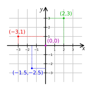
GIS file formats then allow the mathematical parameters that went into georectification to be encoded into the file as well. These are usually a large amount of numbers that describe the equations used and the inputs into all of those equations. Many times you’ll see something like below if you use a tool such as listgeo that can parse the information out of the file format. Note that most formats assume a Cartesian coordinate system running from coordinates (0,0) in the upper left corner to some X and Y to the size of the data set.
listgeo o39102g6.tif Geotiff_Information: Version: 1 Key_Revision: 0.2 Tagged_Information: ModelTiepointTag (2,3): 0 0 0 691331.977 4417194.85 0 ModelPixelScaleTag (1,3): 2.4384 2.4384 0 End_Of_Tags. Keyed_Information: GTModelTypeGeoKey (Short,1): ModelTypeProjected GTRasterTypeGeoKey (Short,1): RasterPixelIsArea ProjectedCSTypeGeoKey (Short,1): PCS_NAD27_UTM_zone_13N PCSCitationGeoKey (Ascii,25): "UTM Zone 13 N with NAD27" End_Of_Keys. End_Of_Geotiff. PCS = 26713 (NAD27 / UTM zone 13N) Projection = 16013 (UTM zone 13N) Projection Method: CT_TransverseMercator ProjNatOriginLatGeoKey: 0.000000 ( 0d 0' 0.00"N) ProjNatOriginLongGeoKey: -105.000000 (105d 0' 0.00"W) ProjScaleAtNatOriginGeoKey: 0.999600 ProjFalseEastingGeoKey: 500000.000000 m ProjFalseNorthingGeoKey: 0.000000 m GCS: 4267/NAD27 Datum: 6267/North American Datum 1927 Ellipsoid: 7008/Clarke 1866 (6378206.40,6356583.80) Prime Meridian: 8901/Greenwich (0.000000/ 0d 0' 0.00"E) Projection Linear Units: 9001/metre (1.000000m) Corner Coordinates: Upper Left ( 691331.977, 4417194.851) (102d45'44.74"W, 39d53' 6.48"N) Lower Left ( 691331.977, 4400540.579) (102d46' 2.23"W, 39d44' 6.68"N) Upper Right ( 704806.576, 4417194.851) (102d36'17.89"W, 39d52'55.15"N) Lower Right ( 704806.576, 4400540.579) (102d36'36.61"W, 39d43'55.41"N) Center ( 698069.276, 4408867.715) (102d41'10.37"W, 39d48'31.03"N)Output of the listgeo command.
From the above output, we can see a few things that describe this image. It came from a USGS DRG that was mathematically warped to a projection (which is why some of them look “tilted” if you’ve looked at a lot of DRGs). Under the ModelTiepointTag key we see several zeros then the numbers 691331.977 and 4417194.85. If you look at the DRG as a two dimensional grid, those numbers represent the latitude and longitude (x, y) coordinates of the upper left pixel in the image. The projection of the DRGs uses meters so the x and y here represent meters in the coordinate system. Under the ModelPixelScaleTag we see another set of numbers, including 2.4384 listed twice. This is the per-pixel scale of the image in meters. So this means that as you increase in the x- or y- direction of the image, each pixel you count up equals 2.4384 meters on the ground. Moving from pixel (0,0) to (10,10) in this case only moves you by a value of 10 on the grid, but would move you 24.384 meters on the ground.
Scale is another issue that may seem counter-intuitive to many people. There are two scales of data that you may hear about: large and small scale. Large scale actually means data that is more detailed than a small scale. The scales do not reference the size of the map but the scale of the map to the Earth. Obviously a 1:1 scale map of the Earth is not feasible since it would have to be as large as the planet. Maps are scaled down to make them much smaller. A common size of a large scale map is 1:25,000 and a small scale map is 1:100,000. The 1:25,000 map is called a large scale because it’s fractional size is larger than that of the 1:100,000 scale map (think of the scales as fractions). A 1:25,000 large scale map does not show as much surface area as the 1:100,000 small scale map, but it shows an area in much more detail than the small scale map does. Think of a large scale map as maps of things like cities, while small scale maps are more along the lines of maps of entire countries.
With the scale discussion out-of-the-way, we then must turn to the usability of geospatial data. Much digital map data was collected from paper maps. Thus, the digital data has a scale where it is most accurate and less accurate at others. Data collected at 1:25,000 scale will be more accurate than data collected at 1:100,000. A GIS allows you to zoom in to the data and in some cases over-zoom past the actual accuracy of the data. Consider data such as a USGS Digital Elevation Model that was collected on a ten meter grid. You can zoom to a view where each pixel on the screen is smaller than ten meters on the ground, but your measurements will not be any more accurate than the ten meter grid you are viewing. Another example is looking at two road maps where one was collected at 1:25,000 and the other at 1:250,000. If you overlay the road maps on to a georeferenced aerial photograph, the 1:25,000 lines will more closely follow actual roads than the ones from the 1:250,000. You cannot expect the 1:250,000 data to be as accurate as the larger scale data, so zooming into a data set will not make the 1:250,000 data any more accurate than the scale where it was captured.
With this out-of-the-way, next time we will start looking at Open Source tools to use the data.