Last time I talked about the problems finding data and in training a machine learning model to classify geologic features from LiDAR.  This time I want to talk about how various libraries can (and cannot) handle 32-bit imagery.  This actually caused most of the technical issues with the project and required multiple work-arounds.

OpenCV and RasterIO

OpenCV is probably the most widely used computer vision library around.  It’s a great library, but it’s written to assume that the entire image can be loaded into memory at once.  To get around this, I had to use the rasterio library as it will read on demand and let you easily read in parts of the image at a time.  To use it with something like Tensorflow, you have to change the data with some code like this:

with rasterio.open(in_file) as src:
    # Read the data as a 3D array (bands, rows, columns)

    # Convert the data type to float32
    data = data.astype(numpy.float32)

    # Transpose the array to match the shape of cv2.imread (rows, columns, bands)
    data = numpy.transpose(data, (1, 2, 0))

    return data
        

Many computer vision algorithms are designed to expect certain types of images, either 8 to 16-bit grayscale or up to 32-bit three channel (such as RGB) images.  OpenCV, one of the most popular, is no different in this aspect .  The mathematical formulas behind these algorithms have certain expectations as well.  Sometimes they can scale to larger numbers of bits, sometimes not.

Finding Areas of Interest

This actually impacts how we search the image for areas of interest.  There are typically two ways to search an image using computer vision: sliding window and selective search.  A sliding window search is a technique used to detect objects or features within an image by moving a window of a fixed size across the image in a systematic manner. Imagine looking through a small square or rectangular frame that you slide over an image, both horizontally and vertically, inspecting every part of the image through this frame. At each position, the content within this window is analyzed to determine whether it contains the object or feature of interest.

Selective Search is an algorithm used in computer vision for efficient object detection. It serves as a preprocessing step that proposes regions in an image that are likely to contain objects. Instead of evaluating every possible location and scale directly through a sliding window, Selective Search intelligently generates a set of region proposals by grouping pixels based on similarity criteria such as color, texture, size, and shape compatibility.

Selective search is more efficient than a sliding window since it returns only “interesting” areas of interest versus a huge number of proposals that a sliding window approach uses.  Selective search in OpenCV is only designed to work with 24 bit images (ie, RGB images with 8 bits per channel).  To use higher-bit data with it, you would have to scale it to 8 bits/channel.  A 32-bit dataset (which includes negative values as these typically indicate no-data areas) can represent 2.15 billion distinct values.  To scale to 8 bits per channel, we would also need to convert it from floating point to 8-bit integer values.  In this case, we can only represent 256 discrete values.  As you can see, this is quite a difference in how many elevations we can differentiate. 

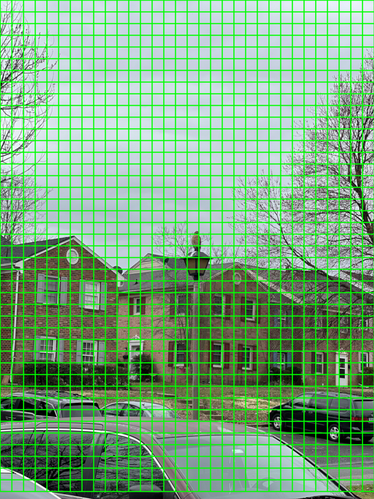
Here’s an example of the areas of interest that a sliding window and image pyramid generates. As you can see, there are a lot of regions of interest that are regularly placed across the image.

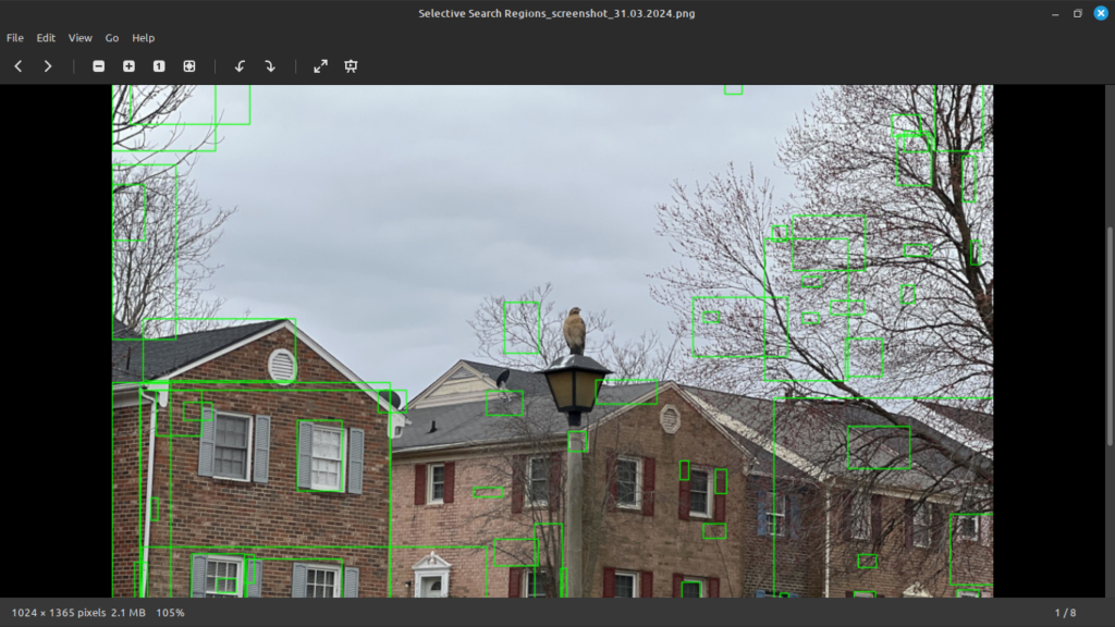
However, selective search is not always perfect.  Below is an example where I ran OpenCV 4’s selective search against an image of mine.  It generated 9,020 proposed areas to search.  I zoomed in to show it did not even show the hawk as a region of interest.

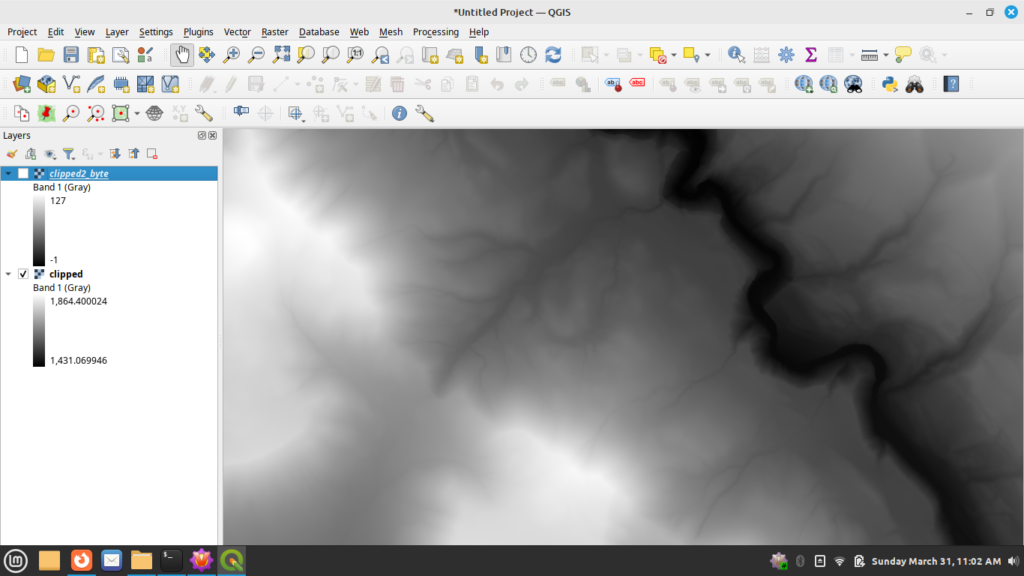
Here’s a clipped version of the input dataset when viewed in QGIS as a 32-bit DEM.  Notice in this case the values range from roughly 1,431 to 1,865.

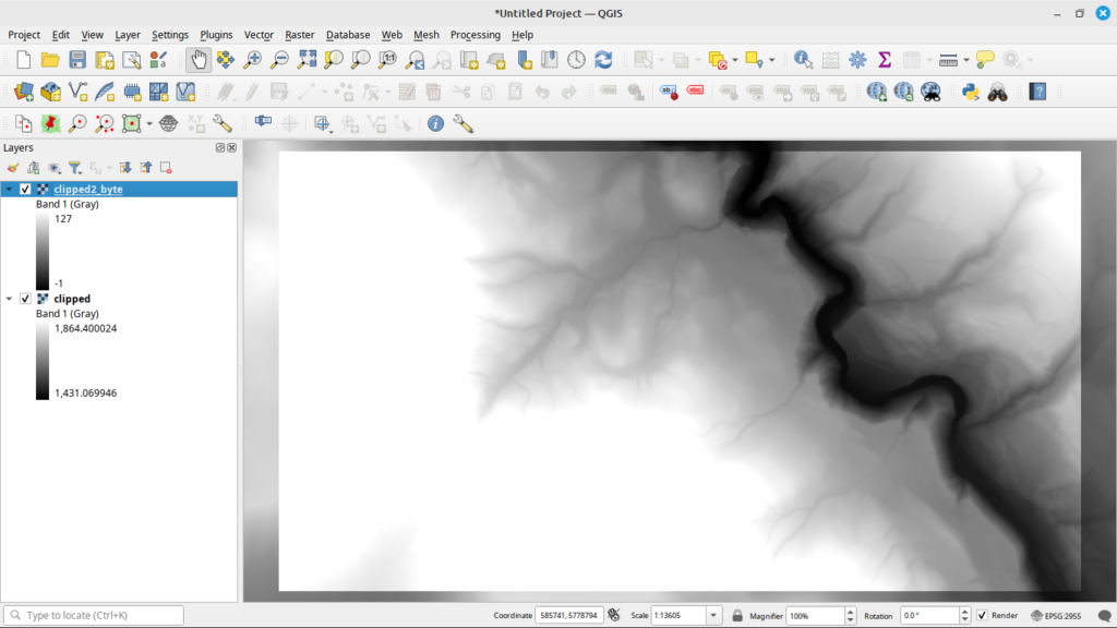
Now here is a version converted to the 8-bit byte format in QGIS.

As you can see, there is quite a difference between the two files.  And before you ask, int8 just results in a black image no matter how I try to adjust the no-data value.

Tensorflow tf.data Pipeline

So to run this, I set up a Tensorflow tf.data pipeline for processing.  My goal was to be able to turn any of the built-in Tensorflow models into a RCNN.  An interesting artifact of using built-in models, Tensorflow, and OpenCV was that the input data actually had to be converted into RGB format.  Yes, this means a 32-bit grayscale image had to become a 32-bit RGB image, which of course greatly increased the memory requirements.  Here’s a code snippet that shows how to use Rasterio, PIL, and numpy to take an input image and convert it so it’s compatible with the built-in Tensorflow models:

def load_and_preprocess_32bit_image(image_bytes: tensorflow.string) -> numpy.ndarray:
    """Helper function to preprocess 32-bit TIFF image
    Args:
       image_bytes (tensorflow.string): Input image bytes
    Returns:
        numpy.ndarray: decoded image
    """

    with rasterio.io.MemoryFile(image_bytes) as memfile:
        with memfile.open() as dataset:
            image = dataset.read()
    
    image = Image.fromarray(image.squeeze().astype('uint32')).convert('RGB')
    image = numpy.array(image)  # Convert to NumPy array
    image = tensorflow.image.resize(image, local_config.IMAGE_SIZE)

    return image

This function takes the 32-bit DEM, loads it, converts it to a 32-bit RGB image, and then converts it to a format that Tensorflow can work with.  

You can then create a function that can use this as part of a tf.data pipeline by defining a function such as this:

def load_and_preprocess_image_train(image_path, label, in_preprocess_input,
                                    is_32bit=False):
    """ Define a function to load, preprocess, and augment the images
    Args:
        image_path (_type_): Path to the input image
        label (_type_): label of the image
        in_reprocess_input: Function from keras to call to preprocess the input
        is_32bit (bool, optional): Is the image a 32 bit greyscale. Defaults to 
                                   False.

    Returns:
     _type_: Pre-processed image and label
    """

    image = tensorflow.io.read_file(image_path)

    if is_32bit:
        image = tensorflow.numpy_function(load_and_preprocess_32bit_image, 
                                          [image],
                                          tensorflow.float32)
    else:
        image = tensorflow.image.decode_image(image, 
                                              channels=3,
                                              expand_animations=False)
        image = tensorflow.image.resize(image, local_config.IMAGE_SIZE)
     
    image = augment_image_train(image)  # Apply data augmentation for training
    image = in_preprocess_input(image)

    return image, label

Lastly, this can then be set up as a part of your tf.data pipeline by using code like this:

# Create a tf.data.Dataset for training data
train_dataset = tf.data.Dataset.from_tensor_slices((train_image_paths, train_labels))
train_dataset = 
    train_dataset.map(lambda path, label:
        image_utilities.load_and_preprocess_image_train(path,
                                                        label,
                                                        preprocess_input,
                                             is_32bit=local_config.USE_TIF,
                                             num_parallel_calls=tf.data.AUTOTUNE)

(Yeah trying to format code on a page in WordPress doesn’t always work so well)

Note I plan on making all of the code public once I make sure the client is cool with that since I was already working on it before taking on their project.  In the meantime, sorry for being a little bit vague.

Training a Model to be a RCNN

Once you have your pipeline set up, it is time to load the built-in model.  In this case I used Xception from Tensorflow and used the pre-trained model to do transfer learning by the standard omit the top layer, freeze the previous layers, then add a new layer on top that learns from the input.

# Load the model without pre-trained weights
base_model = Xception(weights=local_config.PRETRAINED_MODEL, 
                      include_top=False, 
                      input_shape=local_config.IMAGE_SHAPE,
                      classes=num_classes, input_tensor=input_tensor)

# Freeze the base model layers if we're using a pretrained model

if local_config.PRETRAINED_MODEL is not None:
     for layer in base_model.layers:
         layer.trainable = False

# Add a global average pooling layer
x = base_model.output
x = GlobalAveragePooling2D()(x)

# Create the model
predictions = Dense(num_classes, activation='softmax')(x)
model = Model(inputs=base_model.input, outputs=predictions)

In this case, I used Adam as the optimizer as it performed better than something like the stock SGD and I added in two model callbacks.  The first saves the model to disk every time the validation accuracy goes up, and the second stops processing if the accuracy hasn’t improved over a preset number of epochs.  These are actually built-in to Keras and can be set up as follows:

# construct the callback to save only the *best* model to disk based on 
# the validation loss
model_checkpoint = ModelCheckpoint(args["weights"], 
                                   monitor="val_accuracy", 
                                   mode="max", 
                                   save_best_only=True,
                                   verbose=1)

# Add in an early stopping checkpoint so we don't waste our time
early_stop_checkpoint = EarlyStopping(monitor="val_accuracy",
                                      patience=local_config.EPOCHS_EXIT,
                                      restore_best_weights=True)

You can then add them to a list with

model_callbacks = [model_checkpoint, early_stop_checkpoint]

And then pass that into the model.fit function.

After all of this, it was a matter of running the model.  As you can imagine, training took several hours.  Since this has gotten a bit long, I think I’ll go into how I did the detection stages next time.