Stupid LiDAR Tricks Part 2

In this part of the series, I want to go over image salience and how it can be applied to finding “interesting” things in LiDAR.  Image salience (usually used to make salience maps) refers to the ability to identify and highlight the most important or attention-grabbing regions in an image.  It is meant to highlight areas of an image where the human eye would focus first. Salience maps are used to visualize these regions by assigning a salience value to each pixel, indicating its likelihood of being a point of interest. This technique is widely used in computer vision for tasks such as object detection, image segmentation, and visual search.

Background Research

Salience research actually has been going on for decades now.  It began back in the 1950’s where it was a field of psychology and neuroscience that sought to understand how humans perceive and prioritize visual information.  It mainly stayed in the neuroscience and psychology fields until roughly the end of the 1970’s.

In the 1980’s David Marr proposed a computational theory of vision that provided a framework for understanding the stages of how visual systems could process complex scenes.  This can be considered the beginning of trying to recreate how humans prioritized “interesting” parts of an image.  This also can be considered the base upon which later computer science work would be performed.

In the 1990’s the concept of salience maps was proposed to model how the human visual system identifies areas of interest by Itti, Koch, and Neibur.  In 1998 they created one of the first computational models that combined features such as color, intensity, and orientation to calculate areas of interest.  These algorithms added more complex features during the 2000’s.

With the rise of deep learning in the 2010’s, image salience took a turn and began to use CNNs for detection.  By definition, a CNN learns hierarchical features from large datasets and can identify complex patterns in images.  Combined with techniques such as adversarial learning, multi-scale analysis, and attention mechanisms, salience map generation is now more accurate than it has ever been.

CNN Salience Methods

Let us briefly examine how CNNs / deep learning are used in modern times for salience detection:

  • By definition, convolutional layers in a CNN extract local features from an input image.  Early layers in the network capture low-level features such as edges and textures, while later levels in the network capture higher-level features such as actual objects. Multi-scale analysis to process features at different resolutions can also help with salience detection with a CNN.
  • Pooling layers reduce the spatial dimensions of the feature maps.  This makes the computation more efficient and can even provide a form of spatial invariance so that features do not need to be the exact same scale.
  • The final fully-connected layer can then predict the salience map of the image based on the information gathered through the various layers.
  • An encoder-decoder architecture can be used as another extraction mechanism.  Encoders extract features from the image using convolutional layers while gradually reducing the spatial dimensions of the image so that it can increase the depth of the feature maps.
  • Decoders can then reconstruct the salience map from the encoded features.  In this case they may use techniques such as transposed convolutions to upscale the image or “unpooling” to restore the image to the original size.
  • Feature pyramid networks can process an image at multiple scales to gather coarse and fine details and then integrate the information into a final salience map.
  • Finally, generative adversarial networks can be used to produce salience maps by using a generator to create a map and a discriminator to evaluate the quality of the map.  The generator learns to produce more accurate maps over time by attempting to “fool” the discriminator.

Salience Maps

So what is a salience map?  A salience map is a representation that highlights the most important or attention-grabbing regions in an image. It assigns a salience value to each pixel, indicating its likelihood of being a region of interest.  They are the end result of running a salience detector and can be used for:

  • Object detection by finding and localizing objects in an image.
  • Image segmentation by dividing the image into segments or objects based on their salience.
  • Visual search which can be used for things like scene understanding and image retrieval by identifying which areas should have more processing performed.
  • Attention prediction can be used to highlight areas where a person would be most likely to focus their attention.

Why Image Salience?

The last use is what this post is about: automatically finding areas in LiDAR that need to be inspected or to find anomalies in LiDAR.  Imagine you are a large satellite company that collects thousands of images a day.  It would be time consuming for a human to scan all over each image for something of interest.  Salience maps are useful here in that they can help guide a human to places they need to examine.  Potentially, this could be a huge time saver for things like image triage.

LiDAR in raster format provides some challenges, though, for image salience.  For one, LiDAR represents dense, three-dimensional data instead of a normal two-dimensional image.  It requires pre-processing, such as noise reduction and normalization. LiDAR can contain varying point densities and occlusions in the point cloud. This makes LiDAR harder to analyze as we are dealing with a “different” type of image than normal.

Conversion of point data to raster can also make things problematic for salience detection.  LiDAR has several classes, one such class being bare earth.  In most cases, rasterization processes will convert the points to heights based on ground level.  However, in cases of buildings, this would typically have void areas because the laser cannot penetrate a building to find the ground level.   Most tools will fill these voids with a flat ground-level elevation as many people do not wish to see empty areas in their data.  This can make structures on bare earth rasters look similar to things like roads, thus an algorithm might have trouble differentiating the two.

Image Salience and LiDAR Workflow

Since I did not really cover this in the last post, here I will outline a workflow where salience and/or segmentation can be used to help with the processing of large LiDAR datasets (or really any type of raster dataset).

  1. Once the point data has been converted to a raster, salience maps can be generated to identify and extract areas in the imagery that appear to contain meaningful features.
  2. A human can either manually examine the identified areas, or some other complex object detection analysis algorithm can be run against the areas.  This is where the time saving comes into play as only specific parts of the image are examined, not the entire image itself.
  3. Features that are recognized can then be used for higher level tasks, ranging from identifying geographic features to detecting buildings.

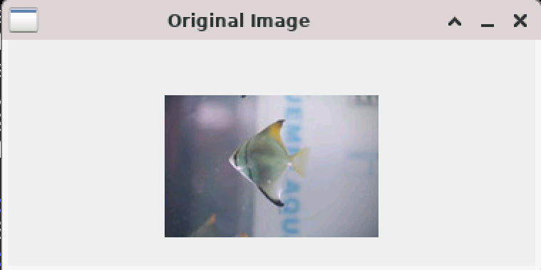
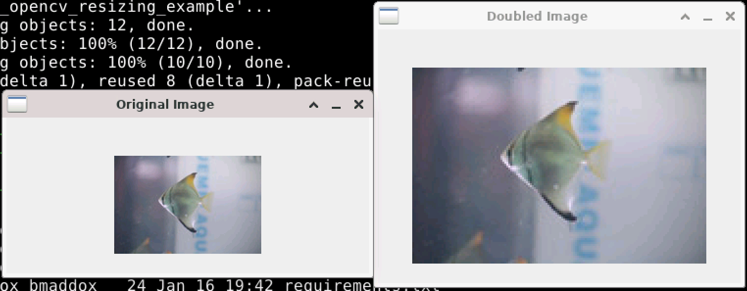
Enough talk and history and theory, let us see how these algorithms actually work.  This source can be found at on github under the salience directory.  This time I made a few changes.  I added a config.py to specify some values for the program to avoid having a lot of command line arguments.   I also have copied the ObjectnessTrainedModel from OpenCV into the salience directory for convenience as not all packaging on Linux actually has the model included.

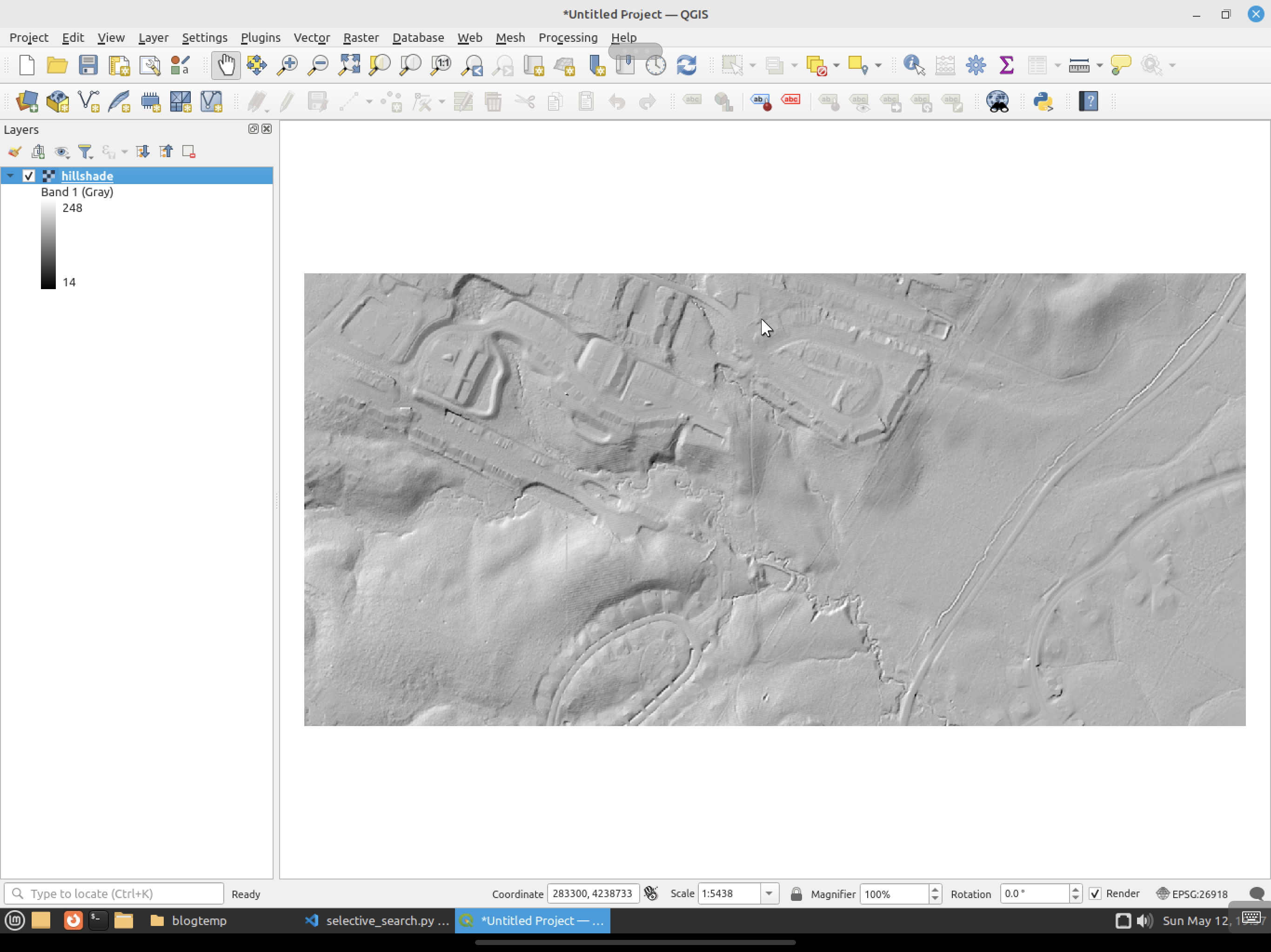
As a reminder, here are the input data sets from the last post (LiDAR and Hill Shade):

First off we will look at the algorithms in the venerable OpenCV package.  OpenCV contains four algorithms for computing salience maps in an image:

  1. Static Saliency Spectral Residual (SFT).  This algorithm works by using the spectral residual of an image’s Fourier transform to generate maps.  It converts the image to the frequency domain by applying the Fourier transform.  It then computes the spectral residual by removing the logarithm of the frequency amplitude spectrum’s average from the logarithm of the amplitude spectrum.  It then performs an inverse Fourier transform to convert the image back into the spatial domain to generate the initial salience map and applies Gaussian filtering to smooth out the maps.
  2. Static Saliency Fine Grained (BMS).  This algorithm uses Boolean maps to simulate how the brain processes an image.  First it performs color quantization on the image to reduce the number of colors so that it can produce larger distinct regions.  It then generates the Boolean maps by thresholding the quantized image at different levels.  Finally, it generates the salience map by combining the various Boolean maps.  Areas that are common across multiple maps are considered to be the salient area of the image.
  3. Motion Salience (ByBinWang).  This is a motion-based algorithm that is used to detect salient areas in a video.  First it calculates the optical flow between consecutive frames to capture the motion information.  It then calculates the magnitude of the motion vectors to find areas with significant movement.  Finally, it generates a salience map by assuming the areas with higher motion magnitudes are the salient parts of the video.
  4. BING Saliencey Detector (BING). This salience detector focuses on predicting the “objectness of image windows, essentially estimating how likely it is that a given window contains an object of interest. It works by learning objectness from a large set of training images using a simple yet effective feature called “Binarized Normed Gradients” (BING).

For our purposes, we will omit the Motion Salience (ByBinWang) method.  It is geared towards videos or image sequences as it calculates motion vectors. 

As this post is already getting long, we will also only look at the OpenCV image processing based methods here.  The next post will take a look at using some of the more modern methods that use deep learning.

Static Saliency Methods

The static salience methods (SFT and BMS) do not produce output bounding boxes around features of an image.  Instead, they produce a floating point image that highlights the important areas of an image.  If you use these, you would normally do something like threshold the images into a binary map so you could find contours, then generate bounding boxes, and so on.

First up is the SFT method.  We will run it now on the LiDAR GeoTIFF.

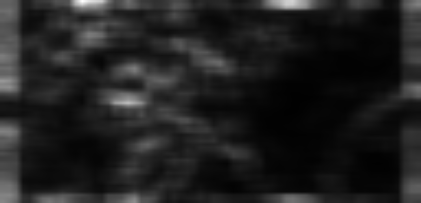
As you can see, when compared to the above original, SFT considers a good part of the image to be unimportant.  There are some areas highlighted, but they do not seem to match up with the features we would be interested in examining.  Next let us try the hill shade TIFF.

For the hill shade, SFT is a bit all over the place.  It picks up a lot of areas that it thinks should be interesting, but again they do not really match up to the places we would be interested in (house outlines, waterways, etc).

Next we try out the BMS method on the LiDAR GeoTIFF.

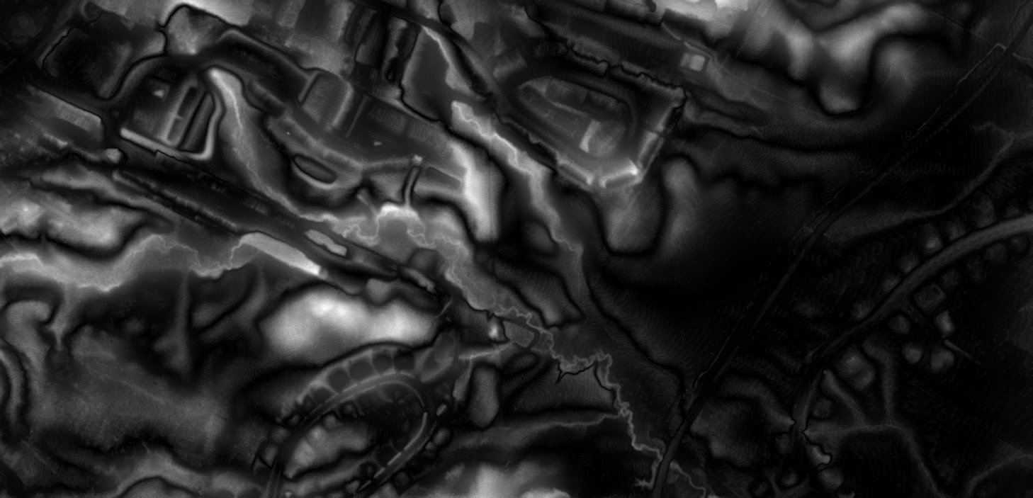
You can see that BMS actually did a decent job with the LiDAR image.  Several of the building footprints have edges that are lighter colored and would show up when thresholded / contoured.  The streams are also highlighted in the image.  The roadway and edges at the lower right side of the image are even picked up a bit.

And now BMS run against the hill shade.

The BMS run against the hill shade TIFF is comparable to the run against the LiDAR GeoTIFF.  Edges of the things we would normally be interested in are highlighted in the image.  It does produce smaller highlighted areas on the hill shade versus the original LiDAR.

The obvious downside to these two techniques is that further processing has to be run to produce actual regions of interest.  You would have to threshold the image into a binary image so you could generate contours.  Then you could convert those contours into bounding boxes via other methods.

Object Saliency Method

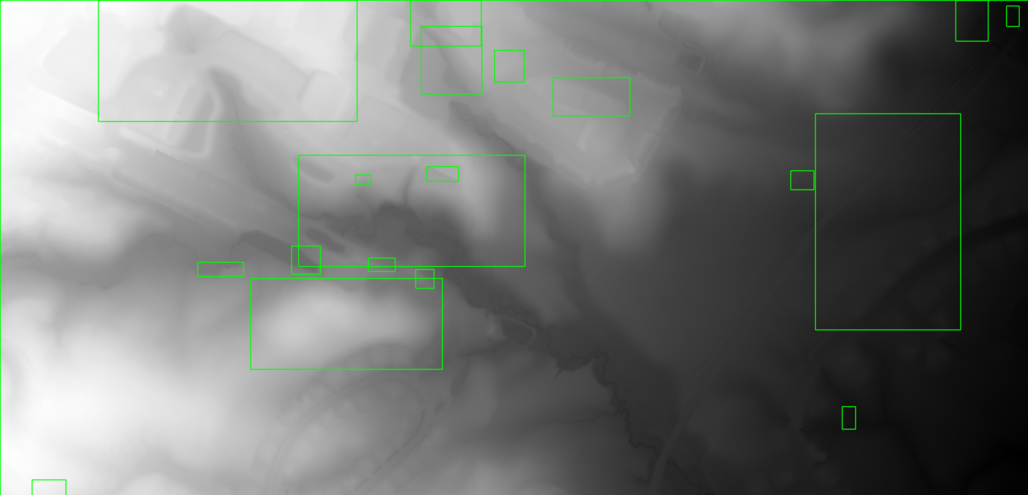
BING is an actual object detector that uses a trained model to find objects in an image.  While not as advanced as many of the modern methods, it does come from 2014 and can be considered the more advanced detection method available for images in OpenCV.  In the config.py file, you can see that with BING, you also have to specify the path to the model that it uses for detection.

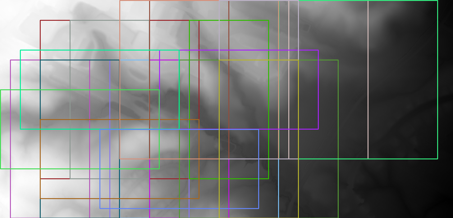
Here we see that BING found larger areas of interest than the static salience methods (SFT and BMS).  While the static methods, especially BMS, did a decent job at detecting individual objects, BING generates larger areas that should be examined.  Finally, let us run BING against the hill shade image.

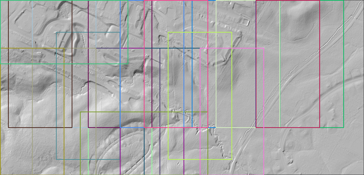
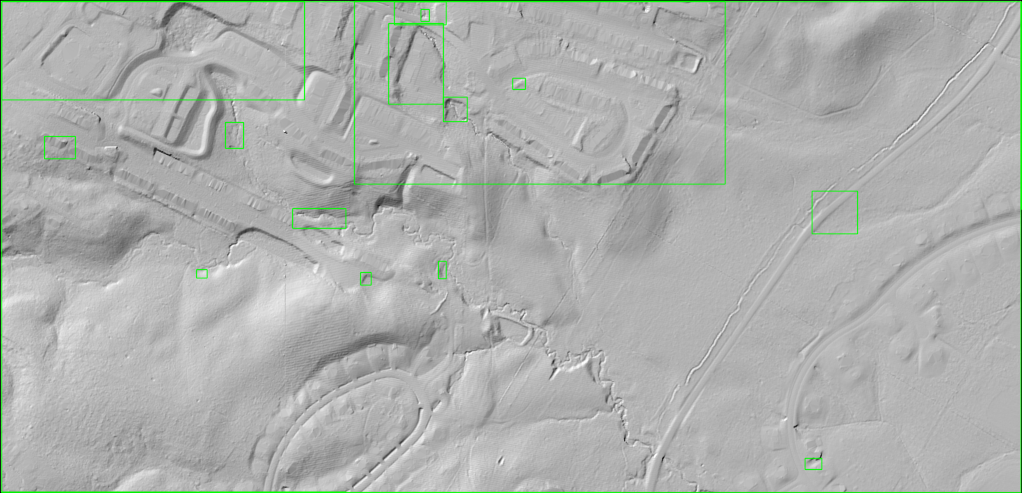
Again we see that BING detected larger areas than the static methods.  The areas are in fact close to what BING found against the LiDAR GeoTIFF.

Results

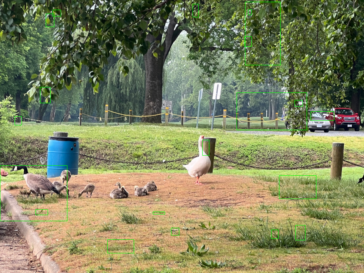
What can we conclude from all of this?  First off, as usual, LiDAR is hard.  Image processing methods to determine image salience can struggle with LiDAR as many areas of interest are not clearly delineated against the background like they would be in an image of your favorite pet.  LiDAR converted to imagery can be chaotic and really pushes traditional image processing methods to the extremes.

Of all of the OpenCV methods to determine salience, I would argue that BMS is the most interesting and does a good job even on the original LiDAR vs the hill shade TIFF.  If we go ahead and threshold the BMS LiDAR image, we can see that it does a good job of guiding us to areas we would find interesting in the LiDAR data.

The BING objectness model fares the worst against the test image.  The areas it identifies are large parts of the image.  If it were a bigger piece of data, it would basically say the entire image is of interest and not do a great job helping to narrow down where exactly a human would need to look.  And in a way this is to be expected.  Finding objects in LiDAR imagery is a difficult task considering how different the imagery is versus normal photographs that most models are trained on.  LiDAR does not often provide an easy separation of foreground versus background.  High-resolution data makes this even worse as things like a river bank can have many different elevation levels.

Next time we will look at modern deep learning-based methods.  How will they fare?  Will they be similar to the BING objectness model and just tell us to examine large swaths of the image?  Or will they work similarly to BMS and guide us to more individual areas.  We will find out next time.

Stupid LiDAR Tricks Part 1 (Segmentation)

My last few posts have been about applying machine learning to try to extract geographic objects in LiDAR.  I think now I would like to go in another direction and talk about ways to help us find anything in LiDAR.  There is a lot of information in LiDAR, and sometimes it would be nice to have a computer help us to find areas we need to examine.

In this case I’m not necessarily just talking about machine learning.  Instead, I am discussing algorithms that can examine an image and identify areas that have something “interesting” in them.  Basically, trying to perform object detection without necessarily determining the object’s identity.

For the next few posts, I think I’ll talk about:

I have a GitHub repository where I’ll stick code that I’m using for this series.

Selective Search (OpenCV)

This first post will talk about selective search, in this specific case, selective search from OpenCV.  Selective search is a segmentation technique used to identify potential regions in an image that might contain objects. In the context of object detection, it can help to quickly narrow down areas of interest before running more complex algorithms. It performs:

  1. Segmentation of the Image: The first step in selective search is to segment the image into multiple small segments or regions. This is typically done using a graph-based segmentation method. The idea is to group pixels together that have similar attributes such as color, texture, size, and shape.
  2. Hierarchical Grouping: After the initial segmentation, selective search employs a hierarchical grouping strategy to merge these small regions into larger ones. It uses a variety of measures to decide which regions to merge, such as color similarity, texture similarity, size similarity, and shape compatibility between the regions. This process is repeated iteratively, resulting in a hierarchical grouping of regions from small to large.
  3. Generating Region Proposals: From this hierarchy of regions, selective search generates region proposals. These proposals are essentially bounding boxes of areas that might contain objects.
  4. Selecting Between Speed and Quality: Selective search allows for configuration between different modes that trade off between speed and the quality (or thoroughness) of the region proposals. “Fast” mode, for example, might be useful in cases of real-time segmentation in videos.  “Quality” is used when processing speed is less important than accuracy.

Additionally. OpenCV allows you to apply various “strategies” to modify the region merging and proposal process.  These strategies are:

  1. Color Strategy: This strategy uses the similarity in color to merge regions. The color similarity is typically measured using histograms of the regions. Regions with similar colors are more likely to be merged under this strategy. This is useful in images where color is a strong indicator of distinct objects.
  2. Texture Strategy: Texture strategy focuses on the texture of the regions. Textures are usually analyzed using local binary patterns or gradient orientations, and regions with similar texture patterns are merged. This strategy is particularly useful in images where texture provides significant information about the objects, such as in natural scenes.
  3. Size Strategy: The size strategy prioritizes merging smaller regions into bigger ones. The idea is to prevent over-segmentation by reducing the number of very small, likely insignificant regions. This strategy tries to control the sizes of the region proposals, balancing between small regions with no areas of interest to large areas that contain multiple areas of interest.
  4. Fill Strategy: This strategy considers how well a region fits within its bounding box. It merges regions that together can better fill a bounding box, minimizing the amount of empty space. The fill strategy is effective in creating more coherent region proposals, especially for objects that are close to being rectangular or square.

Selective Search in Action

Now let us take a look at how selective search works.  This image is of a local celebrity called Gary the Goose.  To follow along, see the selective_search.py code under the selective_search directory in the above GitHub repository.

Gary the Goose

Now let us see how selective search worked on this image:

Selective search on image with all strategies applied.

For this run, selective search was set to quality mode and had all of the strategies applied to it.  As you can see, it found some areas of interest.  It got some of the geese, a street sign, and part of a truck.  But it did not get everything, including the star of the picture.  Now let us try it again, but without applying any of the strategies (comment out line 95).

Default selective search with no strategies applied.

Here we see it did about the same.  Got closer to the large white goose, but still seems to not have picked up a lot in the image.

Selective Search on LiDAR

Now let us try it on a small LiDAR segment.  Here is the sample of a townhome neighborhood.

Small LiDAR clip in QGIS

And here is the best result I could get after running selective search:

Selective search run against LiDAR

As you can see, it did “ok”.  It identified a few areas, but did not pick up on the houses or the small creeks that run through the neighborhood. 

Selective Search on a Hill Shade

Can we do better?  Let us first save the same area as a hillshade GeoTIFF.  Here we take the raw image and apply rendering techniques that simulate how light and shadows would interact with the three dimensional surface, making topographic features in the image easier to see.  You can click some of the links to learn more about it.  Here is the same area where I used QGIS to create and export a hill shade image.

LiDAR as a hill shade.

You can see that the hill shade version makes it easier for a human to pick out features versus the original.  It is easier to spot creeks and the flat areas where buildings are.  Now let us see how selective search handles this file.

Selective Search run against a hill shade.

It did somewhat better.  It identified several of the areas where houses are located, but it still missed all of the others.  It also did not pick up on the creeks that run through the area.

Why Did It Not Work So Well?

Now the question you might have is “Why did selective search do so badly in all of the images?”  Well, this type of segmentation is not actually what we would define as object detection today.  It’s more an image processing operation that builds on techniques that have been around for decades that make use of pixel features to identify areas.

Early segmentation methods that led to selective search typically did the following:

  1. Thresholding: Thresholding segments images based on pixel intensity values. This could be a global threshold applied across the entire image or adaptive thresholds that vary over different sized image regions.
  2. Edge Detection: Edge detectors work by identifying boundaries of objects based on discontinuities in pixel intensities, which often correspond to edges.  Some include a pass to try to connect edges to better identify objects.
  3. Region Growing: This method starts with seed points and “grows” regions by appending neighboring pixels that have similar properties, such as color or texture.
  4. Watershed Algorithm: The watershed algorithm treats the image’s intensity values as a topographic surface, where light areas are high and dark areas are low. “Flooding” the surface from the lowest points segments the image into regions separated by watershed lines.

Selective search came about as a hybrid approach that combined computer vision-based segmentation with strategies to group things together.  Some of these were similarity measures such as color, texture, size, and fill to merge regions together iteratively.  It then introduced a hierarchical grouping that built segments at multiple scales to try to better capture objects in an image.

These techniques do still have their uses.  For example, they can quickly find objects on things like conveyor belts in a manufacturing setting, where the object stands out against a uniform background.  However, they tend to fail when an image is “complicated”, like LiDAR as an example or a white goose that does not easily stand out against the background.  And honestly, they are not really made to work with complex images, especially with LiDAR. These use cases require something more complex than traditional segmentation.

This is way longer now than I expected, so I think I will wrap this up here.  Next time I will talk about another computer vision technique to identify areas of an interest in an image, specifically, image saliency.

Applying Deep Learning to LiDAR Part 3: Algorithms

Last time I talked about the problems finding data and in training a machine learning model to classify geologic features from LiDAR.  This time I want to talk about how various libraries can (and cannot) handle 32-bit imagery.  This actually caused most of the technical issues with the project and required multiple work-arounds.

OpenCV and RasterIO

OpenCV is probably the most widely used computer vision library around.  It’s a great library, but it’s written to assume that the entire image can be loaded into memory at once.  To get around this, I had to use the rasterio library as it will read on demand and let you easily read in parts of the image at a time.  To use it with something like Tensorflow, you have to change the data with some code like this:

with rasterio.open(in_file) as src:
    # Read the data as a 3D array (bands, rows, columns)

    # Convert the data type to float32
    data = data.astype(numpy.float32)

    # Transpose the array to match the shape of cv2.imread (rows, columns, bands)
    data = numpy.transpose(data, (1, 2, 0))

    return data
        

Many computer vision algorithms are designed to expect certain types of images, either 8 to 16-bit grayscale or up to 32-bit three channel (such as RGB) images.  OpenCV, one of the most popular, is no different in this aspect .  The mathematical formulas behind these algorithms have certain expectations as well.  Sometimes they can scale to larger numbers of bits, sometimes not.

Finding Areas of Interest

This actually impacts how we search the image for areas of interest.  There are typically two ways to search an image using computer vision: sliding window and selective search.  A sliding window search is a technique used to detect objects or features within an image by moving a window of a fixed size across the image in a systematic manner. Imagine looking through a small square or rectangular frame that you slide over an image, both horizontally and vertically, inspecting every part of the image through this frame. At each position, the content within this window is analyzed to determine whether it contains the object or feature of interest.

Selective Search is an algorithm used in computer vision for efficient object detection. It serves as a preprocessing step that proposes regions in an image that are likely to contain objects. Instead of evaluating every possible location and scale directly through a sliding window, Selective Search intelligently generates a set of region proposals by grouping pixels based on similarity criteria such as color, texture, size, and shape compatibility.

Selective search is more efficient than a sliding window since it returns only “interesting” areas of interest versus a huge number of proposals that a sliding window approach uses.  Selective search in OpenCV is only designed to work with 24 bit images (ie, RGB images with 8 bits per channel).  To use higher-bit data with it, you would have to scale it to 8 bits/channel.  A 32-bit dataset (which includes negative values as these typically indicate no-data areas) can represent 2.15 billion distinct values.  To scale to 8 bits per channel, we would also need to convert it from floating point to 8-bit integer values.  In this case, we can only represent 256 discrete values.  As you can see, this is quite a difference in how many elevations we can differentiate. 

Here’s an example of the areas of interest that a sliding window and image pyramid generates. As you can see, there are a lot of regions of interest that are regularly placed across the image.

However, selective search is not always perfect.  Below is an example where I ran OpenCV 4’s selective search against an image of mine.  It generated 9,020 proposed areas to search.  I zoomed in to show it did not even show the hawk as a region of interest.

Selective search output run against an image with a hawk.

Here’s a clipped version of the input dataset when viewed in QGIS as a 32-bit DEM.  Notice in this case the values range from roughly 1,431 to 1,865.

QGIS with a clip of the original dataset.

Now here is a version converted to the 8-bit byte format in QGIS.

Same data converted to byte.

As you can see, there is quite a difference between the two files.  And before you ask, int8 just results in a black image no matter how I try to adjust the no-data value.

Tensorflow tf.data Pipeline

So to run this, I set up a Tensorflow tf.data pipeline for processing.  My goal was to be able to turn any of the built-in Tensorflow models into a RCNN.  An interesting artifact of using built-in models, Tensorflow, and OpenCV was that the input data actually had to be converted into RGB format.  Yes, this means a 32-bit grayscale image had to become a 32-bit RGB image, which of course greatly increased the memory requirements.  Here’s a code snippet that shows how to use Rasterio, PIL, and numpy to take an input image and convert it so it’s compatible with the built-in Tensorflow models:

def load_and_preprocess_32bit_image(image_bytes: tensorflow.string) -> numpy.ndarray:
    """Helper function to preprocess 32-bit TIFF image
    Args:
       image_bytes (tensorflow.string): Input image bytes
    Returns:
        numpy.ndarray: decoded image
    """

    with rasterio.io.MemoryFile(image_bytes) as memfile:
        with memfile.open() as dataset:
            image = dataset.read()
    
    image = Image.fromarray(image.squeeze().astype('uint32')).convert('RGB')
    image = numpy.array(image)  # Convert to NumPy array
    image = tensorflow.image.resize(image, local_config.IMAGE_SIZE)

    return image

This function takes the 32-bit DEM, loads it, converts it to a 32-bit RGB image, and then converts it to a format that Tensorflow can work with.  

You can then create a function that can use this as part of a tf.data pipeline by defining a function such as this:


def load_and_preprocess_image_train(image_path, label, in_preprocess_input,
                                    is_32bit=False):
    """ Define a function to load, preprocess, and augment the images
    Args:
        image_path (_type_): Path to the input image
        label (_type_): label of the image
        in_reprocess_input: Function from keras to call to preprocess the input
        is_32bit (bool, optional): Is the image a 32 bit greyscale. Defaults to 
                                   False.

    Returns:
     _type_: Pre-processed image and label
    """

    image = tensorflow.io.read_file(image_path)

    if is_32bit:
        image = tensorflow.numpy_function(load_and_preprocess_32bit_image, 
                                          [image],
                                          tensorflow.float32)
    else:
        image = tensorflow.image.decode_image(image, 
                                              channels=3,
                                              expand_animations=False)
        image = tensorflow.image.resize(image, local_config.IMAGE_SIZE)
     
    image = augment_image_train(image)  # Apply data augmentation for training
    image = in_preprocess_input(image)

    return image, label

Lastly, this can then be set up as a part of your tf.data pipeline by using code like this:

# Create a tf.data.Dataset for training data
train_dataset = tf.data.Dataset.from_tensor_slices((train_image_paths, train_labels))
train_dataset = 
    train_dataset.map(lambda path, label:
        image_utilities.load_and_preprocess_image_train(path,
                                                        label,
                                                        preprocess_input,
                                             is_32bit=local_config.USE_TIF,
                                             num_parallel_calls=tf.data.AUTOTUNE)

(Yeah trying to format code on a page in WordPress doesn’t always work so well)

Note I plan on making all of the code public once I make sure the client is cool with that since I was already working on it before taking on their project.  In the meantime, sorry for being a little bit vague.

Training a Model to be a RCNN

Once you have your pipeline set up, it is time to load the built-in model.  In this case I used Xception from Tensorflow and used the pre-trained model to do transfer learning by the standard omit the top layer, freeze the previous layers, then add a new layer on top that learns from the input.

# Load the model without pre-trained weights
base_model = Xception(weights=local_config.PRETRAINED_MODEL, 
                      include_top=False, 
                      input_shape=local_config.IMAGE_SHAPE,
                      classes=num_classes, input_tensor=input_tensor)

# Freeze the base model layers if we're using a pretrained model

if local_config.PRETRAINED_MODEL is not None:
     for layer in base_model.layers:
         layer.trainable = False

# Add a global average pooling layer
x = base_model.output
x = GlobalAveragePooling2D()(x)

# Create the model
predictions = Dense(num_classes, activation='softmax')(x)
model = Model(inputs=base_model.input, outputs=predictions)

In this case, I used Adam as the optimizer as it performed better than something like the stock SGD and I added in two model callbacks.  The first saves the model to disk every time the validation accuracy goes up, and the second stops processing if the accuracy hasn’t improved over a preset number of epochs.  These are actually built-in to Keras and can be set up as follows:

# construct the callback to save only the *best* model to disk based on 
# the validation loss
model_checkpoint = ModelCheckpoint(args["weights"], 
                                   monitor="val_accuracy", 
                                   mode="max", 
                                   save_best_only=True,
                                   verbose=1)

# Add in an early stopping checkpoint so we don't waste our time
early_stop_checkpoint = EarlyStopping(monitor="val_accuracy",
                                      patience=local_config.EPOCHS_EXIT,
                                      restore_best_weights=True)

You can then add them to a list with

model_callbacks = [model_checkpoint, early_stop_checkpoint]

And then pass that into the model.fit function.

After all of this, it was a matter of running the model.  As you can imagine, training took several hours.  Since this has gotten a bit long, I think I’ll go into how I did the detection stages next time.

Image Processing for Beginners: Image Zooming

Today I’m finally going to finish up the series I started on image processing. The goal of this series is to dispel any myths that algorithms that work on images make things up or do strange, arcane magic. The data is there in the images already, and algorithms that work on them simply make things more visible to a human.

My idea for this originally started when people claimed that zooming in on an image using an iPhone was somehow changing it. The claim (politically motivated) was that it changed the semantic content of the image by zooming in or out. So today I’ll wrap up this series by going over how you zoom an image (or make it larger / smaller).  Note this post will be a bit more technical than the last one as I am including code to demonstrate what I am doing.

Semantic content of an image refers to the meaning or information that the image conveys, such as objects, scenes, actions, attributes, etc. For example, if you take a picture of a cat sitting on a table in your kitchen, then the semantic content would be each of the objects that are in that image (cat, table, kitchen).

Images are resized for you automatically all the time, and you are never aware of it mostly.  Your web browser will scale an image so that it fits on your screen.  Mobile devices scale images such that you can fit them on the device display.  You may even have “pinch to zoom” in on an image so you can see things more clearly.  So ask yourself, when you have zoomed in on an image, do new objects suddenly appear in it?  Does an elephant suddenly appear when you zoom in or out of a picture of your children?  You would have noticed this by now should it happen.

Yes, any time you resize an image you do technically change it, as you have to map pixels from the original to the new size.  However, no resizing operation changes the semantic content of the image.  People have been mapping things and rescaling them long before computers have existed.  Architects, draftsmen, cartographers, and others were transforming and resizing things before electricity was discovered.  Just because a computer does it does not mean that suddenly objects get inserted into the image or that the meaning of the image gets changed.

I’ll be using OpenCV 4 and Python 3. For those unaware, OpenCV is an open source computer vision library that has been around for a long time and is used in thousands of projects. The algorithms in it are some of the best around and have been vetted by experts in the field.  The example image I will be using is a public domain image of a fish as can be seen below.

Public Domain Photo of a Fish

To play along at home, I have the source code for this blog post at https://github.com/briangmaddox/blog_opencv_resizing_example

The first thing we do with our sample image is to load it in using OpenCV, print the dimensions, and then display it.

# Load in our input image
input_image = cv2.imread("1330-sole-fish.jpg")

# Get the dimensions of the original image
height, width, channels = input_image.shape

# Print out the dimensions
print(f"Image Width: {width} Height: {height}")

# Display the original image to the user
cv2.imshow("Original Image", input_image)
cv2.waitKey(0)
cv2.destroyAllWindows()

When we run this code, we see our small fish image in a window:

Image of the fish displayed by OpenCV in a window

Next we will do a “dumb” resize of the image.  Here we double each pixel in the X- and Y-directions.  This has the effect of making the image 2x large, effectively zooming in to the image.

empty_mat = numpy.zeros((height * 2, width * 2, channels), dtype=numpy.uint8)

Here empty_mat is an empty image that has been initialized to all zeroes.  Numpy is a well known array library that OpenCV and other packages are built on.  When OpenCV and Python load an image, they store it in what is basically a three dimensional array.  You can think of this as a box where each red, green, and blue channel of the image is contained in the box.

We do the following loop now to copy the pixel to the output empty_mat:

for y in range(height):
    for x in range(width):
        pixel = input_image[y, x]
        empty_mat[y * 2, x * 2] = pixel
        empty_mat[y * 2, x * 2 + 1] = pixel
        empty_mat[y * 2 + 1, x * 2] = pixel
        empty_mat[y * 2 + 1, x * 2 + 1] = pixel

I used a simple loop and assignments to make it easier to see what I am doing.  This loop simply goes through each row of the input image and copies that pixel to four pixels in the output image, effectively doubling the size and zooming the image.

Now we display both the original image and the doubled one.

cv2.imshow("Original Image", input_image)
cv2.imshow("Doubled image", empty_mat)
cv2.waitKey(0)

cv2.destroyAllWindows()
Both the original image and the doubled image displayed by OpenCV

In the above screenshot, we can see that the image has indeed been “zoomed” in and is now twice the size of the original.  Semantically, both images are equal to each other.  You can see the jaggedness of the fish in the doubled image due to the simplistic nature of the resize.  The main take away from this is that it is still the same image, even if it is larger than the original.

Most applications that let you zoom in or resize images use something a bit smarter than a simple doubling of each pixel.  As you can see with the above images, the simple “doubling” results in a jagged image that becomes less visually pleasing as the zoom multiplier gets larger.  This is because to double an image using the simple method, each pixel becomes four pixels.  Four times larger means eight pixels, and so on.  This method also becomes much more complicated if the zoom factor is not an even multiple of two.

Images today are resized using mathematical interpolations.  Wikipedia defines interpolation as “a type of estimation, a method of constructing (finding) new data new points based on the range of a discrete set of known data points.”  “Ah ha!” you might say, this sounds like things are being made up.  And yes they are, but data is not being made up out of the blue.  Instead, interpolations use existing data to mathematically predict data to fill in the gaps. Google, Apple, and other mapping applications use interpolations to fill in the gaps of your position to display on the screen in-between calculating your exact position using the satellites.  Our brains do it when we reach out to catch a fast ball.  Weather and financial forecasters use it every day.

Interpolations have a long history in mathematics.  The Babylonians were using linear and other interpolations as far back as the 300’s BCE to predict the motions of celestial bodies.  As time has gone on, mathematicians have devised better and more accurate methods of predicting values based on existing ones.  Over time, we have gone from the relatively simplistic piecewise constant interpolations to Gaussian processes.  Each advance has made better and closer predictions to what the missing values actually are.

Consider an example using linear interpolation.  This type of problem is often taught in geometry and other math classes.  Assume that we have points on a two-dimensional XY axis such as below.

Plot of the function y=x with the points (2,2) missing.

Here we see we are given a series of (1,1), (3,3), (4,4), (5,5), (6,6), and (7,7).  This is in fact a plot of the function y = x, except I omitted the point (2,2).  We can eyeball and see that the missing y value for x=2 is in fact 2, but let us go through the math.

The formula for linear interpolation is: .  So if we want to solve for the point where x=2, (x1,y1) will be the point (1,1) and (x2, y2) will be the point (3,3).  Plugging these numbers in we get , which indeed gives us y=2 for x=2.  No magic here, just math.

Other types of interpolations, such as cubic, spline, and so on, also have mathematical equations that calculate new values based on existing values.  This point is important to note.  All interpolations use math to calculate new values based on existing ones.  These interpolations have been used over hundreds of years, and are the basis for many things we use today.  No magic, no guessing, no making things up.  I think we can trust them.

So let us get back to image processing.  OpenCV fortunately can use interpolation to resize an image.  As a reminder, we typically do this so that the image is more pleasing to the eye.  Interpolations give us images that are not blocky as in the case of the simple image doubling technique.  First we will use linear interpolation to double the size of the image

double_width = width * 2
double_height = height * 2
linear_double_image = cv2.resize(input_image, (double_width, double_height), interpolation=cv2.INTER_LINEAR)

# Now display both the original and the linear interpolated image to compare.
cv2.imshow("Original Image", input_image)
cv2.imshow("Linear Interpolated image", linear_double_image)
cv2.waitKey(0)
cv2.destroyAllWindows()

To make things explicit, we set new dimensions to twice the width and height of the image and use linear interpolation to scale the image up.

Original image and a linearly interpolated 2x image displayed with OpenCV

Here we see that the interpolated image is not as blocky as the simple pixel doubling image, meaning that yes the new image is a bit different from the original.  However, nothing new has been added to the image.  It has not been distorted and the same semantic content has been preserved.  We can look at what has happened by examining the coordinates at pixel (0,0) in the original image.

Let us take this farther now.  What happens if we increase to four times the original size?

# Linear interpolation to quad size
quad_width = width * 4
quad_height = height * 4

linear_quad_image = cv2.resize(input_image, (quad_width, quad_height), interpolation=cv2.INTER_LINEAR)

# Now display both the original and the linear interpolated image to compare.
cv2.imshow("Original Image", input_image)
cv2.imshow("Linear Interpolated 4x image", linear_quad_image)
cv2.waitKey(0)
cv2.destroyAllWindows()
Original image and a linearly interpolated 4x image displayed by OpenCV

Again, creating a 4x-size image does not introduce any new objects or change the semantic meaning of the image. You may notice that it looks a bit more blurry than the 2x image.  This is because linear interpolation is a simple process. 

Let us see what it looks like using a more rigorous cubic interpolation to create a 4x image.

# Cubic interpolation
cubic_quad_image = cv2.resize(input_image, (quad_width, quad_height), interpolation=cv2.INTER_CUBIC)

# Now display both the original and the linear interpolated image to compare.
cv2.imshow("Original Image", input_image)
cv2.imshow("Cubic Interpolated 4x image", cubic_quad_image)
cv2.waitKey(0)
cv2.destroyAllWindows()
Original image and the cubic interpolated 4x image displayed by OpenCV

We can see that the image does not have as pronounced blockiness that the linearly interpolated image has.  Yes, it is not exactly the same as the original image as we did not simply double each pixel.  However, the semantic contents of the image are the same, even using a different interpolation method.  We did not introduce anything new into the image by resizing it.  The meaning of the image is the same as it was before.  It is just larger so we can see it better.

It is time to wrap this up as it is a longer post than I intended.  You can see from the above that resizing (or zooming in on) an image does not change the content of the image.  We did not turn the fish into a shark by enlarging it.  We did not add another fish to the image by enlarging it.  

I encourage you to try this on your own at home.  Pull out your phone, take a picture, and then zoom in on it.  Your camera likely takes such a high resolution that displaying it on your screen actually reduces some detail, so that you have to zoom in to see the fine detail in the image.  Ask yourself though, is the meaning of the image changed by zooming in or out on it?  Are they still your children, or did zooming in turn them into something else?

I hope that the next time you hear something in the news about image processing, you realize that every algorithm that does this is just math. It is either math to bring out fine details that you cannot normally see in the case of dark images, or math that makes the image larger so that you can better see the smile on a child.  The content of the image is not changed, it is always semantically the same as the original image.

Image Processing Basics Part 2

Some Examples

Now that we have some of the basics down, let us look at some practical examples of the differences between how the brain sees things versus how a computer does.

Example image of a clear blue sky

The above photo of a part of the sky was taken by my iPhone 13 Pro Max using the native camera application. There were no filters or anything else applied to it. To our eyes, it looks fairly uniform: mainly blue with some lighter blue towards the right where the sun was the day I took the picture. Each pixel of the image represents the light that hit a sensor in the camera, was processed, and saved.

Our brain does not see a number of individual pixels. Instead, we see large splotches of colors. This is one of the shortcuts our brain does to ease the processing burden. If you look around a room, you do not see individual differences between the colors of the wall. Your wall mainly looks like a uniform color. We simply do not have the processing power to break down the inputs from our eyes into every minute part.

A computer, however, does have the ability to “see” an image in all of its different parts. Computers see everything as a number, be it the 1’s and 0’s of binary or color triplets in the RGB color space. If we look at the RGB color cube below, the computer sees all of the pixels in the above image as clustering somewhere around the lower right side of the cube. See the previous link for more information about the RGB color space.

RGB Color cube from wikipedia
RGB Color Cube (Wikimedia Commons contributors, “File:RGB color solid cube.png,” Wikimedia Commons, https://commons.wikimedia.org/w/index.php?title=File:RGB_color_solid_cube.png&oldid=656872808 (accessed April 18, 2023).

In a computer, the above image is loaded and each pixel is in memory in the form of triplets such as (135, 206, 235), which is the code for a color known as sky blue. The computer also does not have to take any shortcuts when it loads the image, meaning that the representation in memory is exactly the same as the image that was saved from the phone.

If we use the OpenCV library to calculate the histogram of the image and then count the number of colors, we in fact find that there are 2,522 unique colors in the picture of the sky. There is no magic here, we just do not have the same precision that a computer does when it comes to examining images or our environment. The big take away here is this: there is more information encoded in pictures or video than what our brains are capable of perceiving. Just because we cannot see certain details in a image does not mean that they are not there.

For another example, consider this image below. The edges look like nothing but black, and all you can really see is out of the window. It is definitely underexposed.

Photo out the window of my wife's grandparents' house.
Photo out the window of my wife’s grandparents’ house.

As mentioned above, a computer is able to detect more than our eyes can. Where we just see black around the edges, there is in fact detail there. We can adjust the exposure on the image to brighten it so that our eyes can see these details.

Above image with the exposure and contrast adjusted

With the exposure turned up (and adjusting the contrast as well), we can additionally see a picture of a bird, some dishes, and some cooking implements. This is not magic, nor is it adding anything to the image that was not already there. Image processing like this does not insert things into an image. It only enhances the details of an image so that they are more detectable to the human eye.

Many times, when image processing is in the news, people sometimes assume that it changing an image, or that it is inserting things that were not originally there. When you edit your images on your phone or tablet, you are manipulating the detail that is already in the image. You can enhance the contrast to make the image “pop.” You can change the color tone of the image to make it appear more warm or more cold to your liking. However, this is simply modifying the information that is already in the image to change how it appears to the human eye.

I am making a big deal about this point as future installments in this series will demonstrate how things actually work while hopefully dispelling certain myths that exist in pop culture. I think next time I will cover zooming in or out of an image (aka, resizing). Does it add something into the image or misrepresent it? We will find out.

Image Processing for the Average Person Part 1 – The Human Visual System

There have been a few things in the news about how computers work with images that I feel are a bit misinformed. I believe these reports mislead the average person about how image processing works. As a huge part of my background, and current business, involve image processing, I thought I would start a series of posts about how computers manipulate images, from zooming in and out, to doing enhancement tasks. I hope to give a decent explanation of things so that you, the reader, will have a better understanding and will be able to separate fiction from facts, politics from reality.

First I want to start with the most import part: the human visual system. It is indeed a miracle of evolution, and works pretty well in helping us to navigate our environment. You might be surprised to find, however, that it’s not exactly as good as you might think it is.

Our Vision System Makeup

The Human VisuaL Pathway, Miquel Perello Nieto, CC BY-SA 4.0 https://creativecommons.org/licenses/by-sa/4.0, via Wikimedia Commons

A simplified view of our visual system is that it is made up of the eye, which can be thought of as a camera, the optic nerve (USB cable), and the brain (computer). In reality, there are many more parts to this, including multiple parts of the eye, different parts of the brain that detect and react to different parts of what the eye sees, and so on. There are numerous articles online that break this down into much more detail, but for this series it is enough to use the simplistic point of view.

Physical Characteristics

The specs of our visual system are roughly what is listed below:

  • Much like a physical camera, the performance of our eyes depends a lot on age and the quality of the parts. As we get older, our lens stops performing as well, we get eye floaters, and other issues.
  • Our eyes have receptors in the back that fire when light hits them.
  • Each eye has what is known as a blind spot located where the optic nerve passes through the optic disc. There are no light receptors here so it no data can go to the brain from this area. Do not feel bad, though, as all vertebrate eyes have a blind spot, so it is not just us humans.
  • Our eyes can adapt to a range of intensity of almost ten orders of magnitude. It cannot operate over all of this range simultaneously, however.
  • While we think our eyes see the same all over, we actually only see clearly over the fovea. The fovea is the part of the eye that receives light from the central two degrees of our field of view. To get an idea about how small this is, imagine holding a quarter or half dollar coin at your arm’s length.
  • It is actually hard to assign a resolution such as 1920×1080 to the human eye, as resolutions are dependent on characteristics like sensor size, pixel density, and so on. Instead, we need to think about it in terms of how many pixels make up our vision. Our total field of vision can be thought of as having around 580 megapixels of resolution. Keep in mind that this represents our total field of vision, and that our fovea is the part of the eye that clearly focuses light.
  • Our fovea can be thought of as only being around seven megapixels of resolution. Our eyes are constantly in motion so create our field of view by sending in multiple snapshots to the brain to create our sight. Estimates are that outside of the fovea, the rest of the snapshot is thought to only contain about one megapixel of data.
  • If we want to think in terms of a video frame rate, our eyes and brains can only process around a paltry fifteen frames a second. We see an illusion of motion due to a concept called beta movement. This is chiefly due to how long the visual cortex stores data coming in from the eyes.

Processing Characteristics

Once light coming into our eyes passes to the brain, it runs into several systems that work up to us cognitively recognizing what we are looking at. Again, I am not going to get into the weeds here as there is already plenty of information online about what goes on in portions of the brain such as the visual cortex.

The comparison to a simple camera breaks down here, as our brain has a final say in what we actually see. Parts of the brain work together to help us understand the different parts of the chair, but in the end we decide “Oh I’m looking at a chair.” The brain can also be fooled in its interpretation of what the physical part of the visual system is seeing.

Two profiles or a vase? - Ian Remsen, CC0, via Wikimedia Commons
Two profiles or a vase? – Ian Remsen, CC0, via Wikimedia Commons

An example of this trickery is in optical illusions. This happens when the brain tries to fill in the gaps of information that it needs to decide. It can also misinterpret geometrical properties of an object that results in an incorrect analysis.

The brain merges an amalgamation of what the eyes see into our view of the world. Our eyes are constantly moving, making minute changes to what they are focusing on as we are looking at something. The brain interpolates incoming information to fill in the gaps from parts of the eye like the blind spot and faulty receptors. This means that the brain does a lot of processing to generate what we perceive as our default field of view.

This is a lot of information, so the brain takes as many shortcuts as it can in processing our visual data. We may have a super computer on our necks, but it can only process so much so quickly. This is where comparing our eyes to a camera breaks down as a lot of what we see is based on perception versus physical processing. Our brains cannot store every “megapixel” of what we see in our memories either, so we remember things more as concepts and objects than each individual component of a picture. We simply do not have enough storage to keep everything in our memory.

This finely balanced system of optics and processing and simplification can also break down. We see fast motion as being blurred, or, well, having motion blur. This is because our eyes cannot move fast enough and our brain cannot process fast enough to see individual images, so the brain adds in blur so we understand something is in motion. Now, on a sufficiently high frame rate high definition display, objects are captured without blur, which can mess with our brain’s processing and cause us to have a headache. Think of it as our brain trying to keep up and basically having a blue screen.

This is probably a good place to wrap this up today. I mainly wanted to give a quick explanation of how we see the world to demonstrate that our own eyes are not always perfect, and that a lot goes on behind the scenes to enable our vision.

Next time I’ll start going into some specifics, including showing the difference between what we see and what a computer might see.