Some Background on Natural Language Processing – Part 1: English

I thought I would switch topics and start to talk about things like Large Language Models and how they could be applied to things like Geographic Information System (GIS) data.  To do this, I think first it would be good to talk about the basis for some of these tools, such as natural language processing (NLP).  

NLP is the basis for tools such as LLMs and even the ability to extract information from GIS data such as people, places, and things.  As such, I feel it is important to understand NLP as it provides a lot of value to GIS information as well as advanced processing of such information.

Some background about English

Before I dive into how NLP works, I first want to talk about the English language and how it relates to NLP.  This will give some background about why NLP is hard and how far we have come over the years.  So we will have a bit of a history lesson.  I love history and I finally have a reason to blog about it.  Next post we will dig into the background of how NLP used to work and how it works today.

What is the English Language?

First off, English is a horrible language.  It is a West Germanic language that is a part of the Indo-European language family.  It is a mashup of several different languages and continues to evolve almost yearly with new terms being added.  It got its start in what is now the UK prior to the fifth century when it was inhabited Celtic-speaking peoples.  Then came the Romans who tried to enforce Latin, but the natives said no for the most part.

Old English

Next came the Anglo-Saxons who came to Britain from the area around the northwest of modern Germany.  These Anglo-Saxon travelers brought their Ingvaeonic languages to Britain, displaced the Celts, and then started what we now call Old English.  Then while Old English was forming, we throw in some influence form the Vikings who invaded off and on and imparted some of their Norse words into the mix.  Then, to top things off, we had four known variants of the language that developed in Britain.

An example comes from Beowulf what was written around 1000 AD and here is the first line of it:

HWÆT:  WE GAR-DENA IN GEARDAGUM (So. The Spear-Danes in days gone by)

Middle English

Then came the Normans in 1066.  The Normans at the time spoke Anglo-Norman / Anglo-Norman French / Old French.  This became the language of the upper class and the courts of the time.  English then brought in some of the French words to add to the mix.  However, this did simplify the grammar of the language a bit.  This then went on to give us Middle English.  An example of this is found in The Canterbury Tales, where one of my high school English teachers made us memorize the first verse of it and scarred me for life.

Whan that Aprill with his shoures soote (When April with its sweet-smelling showers)

Early Modern English

Then we move on to Early Modern English that started to take root in the 15th to 17th centuries, better known as the Renaissance.  Here we decided to throw in some Latin, Greek, and even more French words for good measure.  The good news is that we started to simplify the grammar even more.  During this time, English went through the Great Vowel Shift.  This change modified how long vowels were pronounced and thus threw in some spelling changes.  The results of this shift have had wide-ranging impacts, including the basis for spelling and pronunciation mismatches in Modern English.  Plus the English and French began their love/hate relationship so it is possible that some anti-French sentiment caused some words to be modified to lose their influence, so to speak.  This was also the language used by Shakespeare who also added words to the language.  Here is an example of what the Lord’s Prayer would have looked like during this period.

Our father which art in heauen, hallowed be thy name. Thy kingdome come. Thy will be done, in earth, as it is in heauen.

Modern and Contemporary English

We finally arrive at Modern English which started in the 17th century and continues on today.  Thanks to the British Empire, English spread globally.  This global contact ended up adding more word to the language.  It went on to become the language of business, science, and diplomacy.

Then you may have heard of a bit of a spat between the British and a bunch of upstart colonies that formed the United States.  As time went on, American English began to differ a bit from British English, mainly in some spellings and different words for things (a car’s hood vs a car’s bonnet).  As the empire fell, we also got various dialects of English including Canadian and Australian English.

A Language that Confuses Native Speakers

This brings us to Contemporary English, a language with a large history of change and influences and words from various cultures.  Unlike Latin-based languages, it really does not follow many rules.  It tends to reuse words with different tenses and even different parts of speech.  The same word can have a lot of different and even non-related meanings.  Consider this, a perfectly valid sentence today:

I banked(1) on the advice from my friend and ended up making a lot of bank(2) by playing the bank(3) of slot machines at the casino.  To keep it safe, I decided to take it to the new bank(4) that they built on the south bank(5) of the river.

As a native American English speaker, this makes me want to cry.  This is why it is so hard for non-native English speakers to learn the language.  Let us look at the abomination that I just wrote.  The word bank is used as a:

  1. Verb: meaning to rely on
  2. Noun (slang really): meaning money
  3. Noun: meaning a row of similar items
  4. Noun: meaning a place to store things for later use
  5. Noun: sloping raised land near a river

Imagine you are someone trying to learn English and you come across that sentence.  Your head would explode.  Think about how hard it would be to figure out what was actually being said.  Note that I could have added another verb use by saying something like “On the way there, I had to bank to the left in my car to get in the proper lane.”  Thankfully I felt bad enough making the above sentence in the first place.

Now imagine a computer trying to parse this.  Remember that a computer is a glorified calculator.  Admittedly that sentence was made up to be a specific edge case, but it illustrates the point that if a human would have trouble understanding something, you can be sure that I computer will too.  And NLP has come a long way and these days would actually be able to make use of that sentence.

Distinguishing the meaning of the same word used in many different contexts has been, and continues to be, one of the primary reasons that getting NLP right has been so hard.  We have ended up with many historic and structural complexities that have led to the language today. 

Historically, most NLP research has been done on the English language due to its dominance in commerce and the link.  NLP into other languages is working to catch up, but for these blog posts I am going to consider that to be out of scope since, well, I do not speak those languages.

And to add in another complication, research and methods of NLP for the English languages do not exactly work well for other languages.  Each language has its own grammar and usage.  Some languages such as Spanish and French (Romance Languages) are similar at least.  But it is basically an apples to oranges comparison to try to apply English NLP principals to something like an Asian language.

Conclusion

I think I will leave things here for today.  Next time I will go into the history of how NLP worked in the past before moving on to how it works today.

Stupid LiDAR Tricks Part 2

In this part of the series, I want to go over image salience and how it can be applied to finding “interesting” things in LiDAR.  Image salience (usually used to make salience maps) refers to the ability to identify and highlight the most important or attention-grabbing regions in an image.  It is meant to highlight areas of an image where the human eye would focus first. Salience maps are used to visualize these regions by assigning a salience value to each pixel, indicating its likelihood of being a point of interest. This technique is widely used in computer vision for tasks such as object detection, image segmentation, and visual search.

Background Research

Salience research actually has been going on for decades now.  It began back in the 1950’s where it was a field of psychology and neuroscience that sought to understand how humans perceive and prioritize visual information.  It mainly stayed in the neuroscience and psychology fields until roughly the end of the 1970’s.

In the 1980’s David Marr proposed a computational theory of vision that provided a framework for understanding the stages of how visual systems could process complex scenes.  This can be considered the beginning of trying to recreate how humans prioritized “interesting” parts of an image.  This also can be considered the base upon which later computer science work would be performed.

In the 1990’s the concept of salience maps was proposed to model how the human visual system identifies areas of interest by Itti, Koch, and Neibur.  In 1998 they created one of the first computational models that combined features such as color, intensity, and orientation to calculate areas of interest.  These algorithms added more complex features during the 2000’s.

With the rise of deep learning in the 2010’s, image salience took a turn and began to use CNNs for detection.  By definition, a CNN learns hierarchical features from large datasets and can identify complex patterns in images.  Combined with techniques such as adversarial learning, multi-scale analysis, and attention mechanisms, salience map generation is now more accurate than it has ever been.

CNN Salience Methods

Let us briefly examine how CNNs / deep learning are used in modern times for salience detection:

  • By definition, convolutional layers in a CNN extract local features from an input image.  Early layers in the network capture low-level features such as edges and textures, while later levels in the network capture higher-level features such as actual objects. Multi-scale analysis to process features at different resolutions can also help with salience detection with a CNN.
  • Pooling layers reduce the spatial dimensions of the feature maps.  This makes the computation more efficient and can even provide a form of spatial invariance so that features do not need to be the exact same scale.
  • The final fully-connected layer can then predict the salience map of the image based on the information gathered through the various layers.
  • An encoder-decoder architecture can be used as another extraction mechanism.  Encoders extract features from the image using convolutional layers while gradually reducing the spatial dimensions of the image so that it can increase the depth of the feature maps.
  • Decoders can then reconstruct the salience map from the encoded features.  In this case they may use techniques such as transposed convolutions to upscale the image or “unpooling” to restore the image to the original size.
  • Feature pyramid networks can process an image at multiple scales to gather coarse and fine details and then integrate the information into a final salience map.
  • Finally, generative adversarial networks can be used to produce salience maps by using a generator to create a map and a discriminator to evaluate the quality of the map.  The generator learns to produce more accurate maps over time by attempting to “fool” the discriminator.

Salience Maps

So what is a salience map?  A salience map is a representation that highlights the most important or attention-grabbing regions in an image. It assigns a salience value to each pixel, indicating its likelihood of being a region of interest.  They are the end result of running a salience detector and can be used for:

  • Object detection by finding and localizing objects in an image.
  • Image segmentation by dividing the image into segments or objects based on their salience.
  • Visual search which can be used for things like scene understanding and image retrieval by identifying which areas should have more processing performed.
  • Attention prediction can be used to highlight areas where a person would be most likely to focus their attention.

Why Image Salience?

The last use is what this post is about: automatically finding areas in LiDAR that need to be inspected or to find anomalies in LiDAR.  Imagine you are a large satellite company that collects thousands of images a day.  It would be time consuming for a human to scan all over each image for something of interest.  Salience maps are useful here in that they can help guide a human to places they need to examine.  Potentially, this could be a huge time saver for things like image triage.

LiDAR in raster format provides some challenges, though, for image salience.  For one, LiDAR represents dense, three-dimensional data instead of a normal two-dimensional image.  It requires pre-processing, such as noise reduction and normalization. LiDAR can contain varying point densities and occlusions in the point cloud. This makes LiDAR harder to analyze as we are dealing with a “different” type of image than normal.

Conversion of point data to raster can also make things problematic for salience detection.  LiDAR has several classes, one such class being bare earth.  In most cases, rasterization processes will convert the points to heights based on ground level.  However, in cases of buildings, this would typically have void areas because the laser cannot penetrate a building to find the ground level.   Most tools will fill these voids with a flat ground-level elevation as many people do not wish to see empty areas in their data.  This can make structures on bare earth rasters look similar to things like roads, thus an algorithm might have trouble differentiating the two.

Image Salience and LiDAR Workflow

Since I did not really cover this in the last post, here I will outline a workflow where salience and/or segmentation can be used to help with the processing of large LiDAR datasets (or really any type of raster dataset).

  1. Once the point data has been converted to a raster, salience maps can be generated to identify and extract areas in the imagery that appear to contain meaningful features.
  2. A human can either manually examine the identified areas, or some other complex object detection analysis algorithm can be run against the areas.  This is where the time saving comes into play as only specific parts of the image are examined, not the entire image itself.
  3. Features that are recognized can then be used for higher level tasks, ranging from identifying geographic features to detecting buildings.

Enough talk and history and theory, let us see how these algorithms actually work.  This source can be found at on github under the salience directory.  This time I made a few changes.  I added a config.py to specify some values for the program to avoid having a lot of command line arguments.   I also have copied the ObjectnessTrainedModel from OpenCV into the salience directory for convenience as not all packaging on Linux actually has the model included.

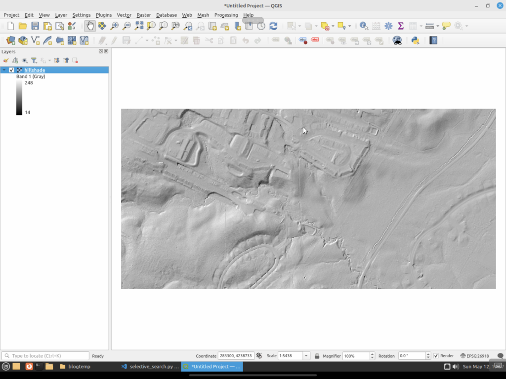
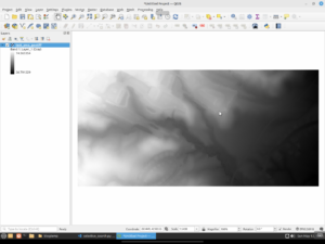
As a reminder, here are the input data sets from the last post (LiDAR and Hill Shade):

First off we will look at the algorithms in the venerable OpenCV package.  OpenCV contains four algorithms for computing salience maps in an image:

  1. Static Saliency Spectral Residual (SFT).  This algorithm works by using the spectral residual of an image’s Fourier transform to generate maps.  It converts the image to the frequency domain by applying the Fourier transform.  It then computes the spectral residual by removing the logarithm of the frequency amplitude spectrum’s average from the logarithm of the amplitude spectrum.  It then performs an inverse Fourier transform to convert the image back into the spatial domain to generate the initial salience map and applies Gaussian filtering to smooth out the maps.
  2. Static Saliency Fine Grained (BMS).  This algorithm uses Boolean maps to simulate how the brain processes an image.  First it performs color quantization on the image to reduce the number of colors so that it can produce larger distinct regions.  It then generates the Boolean maps by thresholding the quantized image at different levels.  Finally, it generates the salience map by combining the various Boolean maps.  Areas that are common across multiple maps are considered to be the salient area of the image.
  3. Motion Salience (ByBinWang).  This is a motion-based algorithm that is used to detect salient areas in a video.  First it calculates the optical flow between consecutive frames to capture the motion information.  It then calculates the magnitude of the motion vectors to find areas with significant movement.  Finally, it generates a salience map by assuming the areas with higher motion magnitudes are the salient parts of the video.
  4. BING Saliencey Detector (BING). This salience detector focuses on predicting the “objectness of image windows, essentially estimating how likely it is that a given window contains an object of interest. It works by learning objectness from a large set of training images using a simple yet effective feature called “Binarized Normed Gradients” (BING).

For our purposes, we will omit the Motion Salience (ByBinWang) method.  It is geared towards videos or image sequences as it calculates motion vectors. 

As this post is already getting long, we will also only look at the OpenCV image processing based methods here.  The next post will take a look at using some of the more modern methods that use deep learning.

Static Saliency Methods

The static salience methods (SFT and BMS) do not produce output bounding boxes around features of an image.  Instead, they produce a floating point image that highlights the important areas of an image.  If you use these, you would normally do something like threshold the images into a binary map so you could find contours, then generate bounding boxes, and so on.

First up is the SFT method.  We will run it now on the LiDAR GeoTIFF.

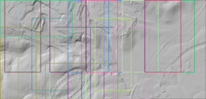
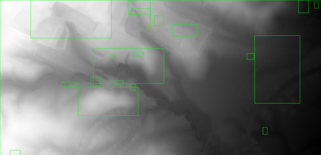
As you can see, when compared to the above original, SFT considers a good part of the image to be unimportant.  There are some areas highlighted, but they do not seem to match up with the features we would be interested in examining.  Next let us try the hill shade TIFF.

For the hill shade, SFT is a bit all over the place.  It picks up a lot of areas that it thinks should be interesting, but again they do not really match up to the places we would be interested in (house outlines, waterways, etc).

Next we try out the BMS method on the LiDAR GeoTIFF.

You can see that BMS actually did a decent job with the LiDAR image.  Several of the building footprints have edges that are lighter colored and would show up when thresholded / contoured.  The streams are also highlighted in the image.  The roadway and edges at the lower right side of the image are even picked up a bit.

And now BMS run against the hill shade.

The BMS run against the hill shade TIFF is comparable to the run against the LiDAR GeoTIFF.  Edges of the things we would normally be interested in are highlighted in the image.  It does produce smaller highlighted areas on the hill shade versus the original LiDAR.

The obvious downside to these two techniques is that further processing has to be run to produce actual regions of interest.  You would have to threshold the image into a binary image so you could generate contours.  Then you could convert those contours into bounding boxes via other methods.

Object Saliency Method

BING is an actual object detector that uses a trained model to find objects in an image.  While not as advanced as many of the modern methods, it does come from 2014 and can be considered the more advanced detection method available for images in OpenCV.  In the config.py file, you can see that with BING, you also have to specify the path to the model that it uses for detection.

Here we see that BING found larger areas of interest than the static salience methods (SFT and BMS).  While the static methods, especially BMS, did a decent job at detecting individual objects, BING generates larger areas that should be examined.  Finally, let us run BING against the hill shade image.

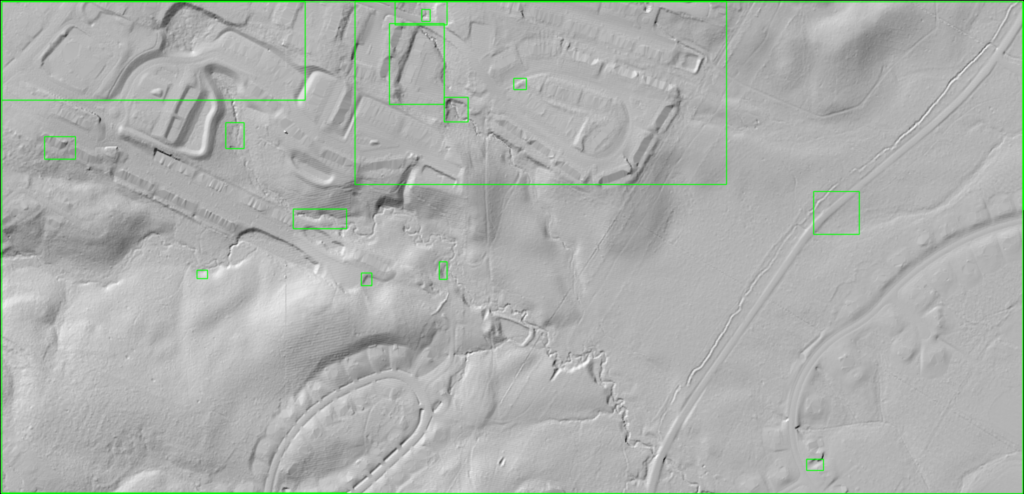
Again we see that BING detected larger areas than the static methods.  The areas are in fact close to what BING found against the LiDAR GeoTIFF.

Results

What can we conclude from all of this?  First off, as usual, LiDAR is hard.  Image processing methods to determine image salience can struggle with LiDAR as many areas of interest are not clearly delineated against the background like they would be in an image of your favorite pet.  LiDAR converted to imagery can be chaotic and really pushes traditional image processing methods to the extremes.

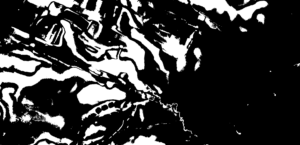
Of all of the OpenCV methods to determine salience, I would argue that BMS is the most interesting and does a good job even on the original LiDAR vs the hill shade TIFF.  If we go ahead and threshold the BMS LiDAR image, we can see that it does a good job of guiding us to areas we would find interesting in the LiDAR data.

The BING objectness model fares the worst against the test image.  The areas it identifies are large parts of the image.  If it were a bigger piece of data, it would basically say the entire image is of interest and not do a great job helping to narrow down where exactly a human would need to look.  And in a way this is to be expected.  Finding objects in LiDAR imagery is a difficult task considering how different the imagery is versus normal photographs that most models are trained on.  LiDAR does not often provide an easy separation of foreground versus background.  High-resolution data makes this even worse as things like a river bank can have many different elevation levels.

Next time we will look at modern deep learning-based methods.  How will they fare?  Will they be similar to the BING objectness model and just tell us to examine large swaths of the image?  Or will they work similarly to BMS and guide us to more individual areas.  We will find out next time.

Stupid LiDAR Tricks Part 1 (Segmentation)

My last few posts have been about applying machine learning to try to extract geographic objects in LiDAR.  I think now I would like to go in another direction and talk about ways to help us find anything in LiDAR.  There is a lot of information in LiDAR, and sometimes it would be nice to have a computer help us to find areas we need to examine.

In this case I’m not necessarily just talking about machine learning.  Instead, I am discussing algorithms that can examine an image and identify areas that have something “interesting” in them.  Basically, trying to perform object detection without necessarily determining the object’s identity.

For the next few posts, I think I’ll talk about:

I have a GitHub repository where I’ll stick code that I’m using for this series.

Selective Search (OpenCV)

This first post will talk about selective search, in this specific case, selective search from OpenCV.  Selective search is a segmentation technique used to identify potential regions in an image that might contain objects. In the context of object detection, it can help to quickly narrow down areas of interest before running more complex algorithms. It performs:

  1. Segmentation of the Image: The first step in selective search is to segment the image into multiple small segments or regions. This is typically done using a graph-based segmentation method. The idea is to group pixels together that have similar attributes such as color, texture, size, and shape.
  2. Hierarchical Grouping: After the initial segmentation, selective search employs a hierarchical grouping strategy to merge these small regions into larger ones. It uses a variety of measures to decide which regions to merge, such as color similarity, texture similarity, size similarity, and shape compatibility between the regions. This process is repeated iteratively, resulting in a hierarchical grouping of regions from small to large.
  3. Generating Region Proposals: From this hierarchy of regions, selective search generates region proposals. These proposals are essentially bounding boxes of areas that might contain objects.
  4. Selecting Between Speed and Quality: Selective search allows for configuration between different modes that trade off between speed and the quality (or thoroughness) of the region proposals. “Fast” mode, for example, might be useful in cases of real-time segmentation in videos.  “Quality” is used when processing speed is less important than accuracy.

Additionally. OpenCV allows you to apply various “strategies” to modify the region merging and proposal process.  These strategies are:

  1. Color Strategy: This strategy uses the similarity in color to merge regions. The color similarity is typically measured using histograms of the regions. Regions with similar colors are more likely to be merged under this strategy. This is useful in images where color is a strong indicator of distinct objects.
  2. Texture Strategy: Texture strategy focuses on the texture of the regions. Textures are usually analyzed using local binary patterns or gradient orientations, and regions with similar texture patterns are merged. This strategy is particularly useful in images where texture provides significant information about the objects, such as in natural scenes.
  3. Size Strategy: The size strategy prioritizes merging smaller regions into bigger ones. The idea is to prevent over-segmentation by reducing the number of very small, likely insignificant regions. This strategy tries to control the sizes of the region proposals, balancing between small regions with no areas of interest to large areas that contain multiple areas of interest.
  4. Fill Strategy: This strategy considers how well a region fits within its bounding box. It merges regions that together can better fill a bounding box, minimizing the amount of empty space. The fill strategy is effective in creating more coherent region proposals, especially for objects that are close to being rectangular or square.

Selective Search in Action

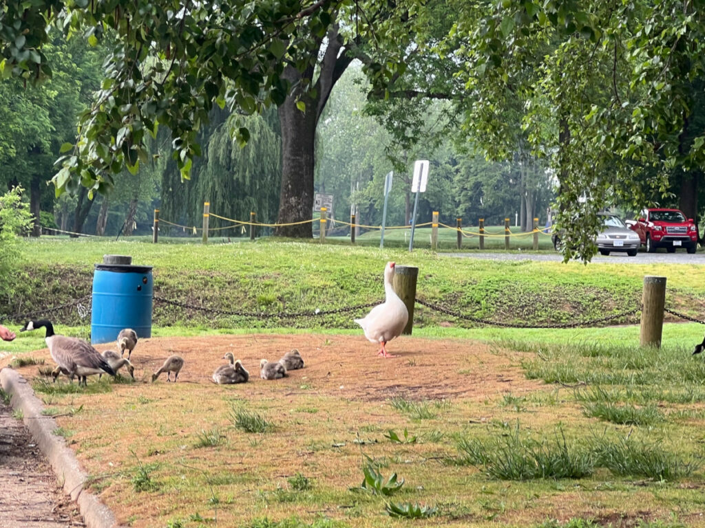
Now let us take a look at how selective search works.  This image is of a local celebrity called Gary the Goose.  To follow along, see the selective_search.py code under the selective_search directory in the above GitHub repository.

Gary the Goose

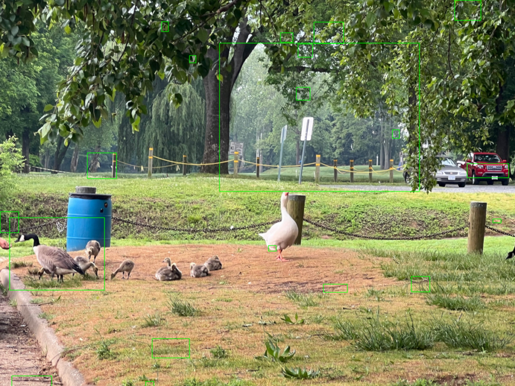
Now let us see how selective search worked on this image:

Selective search on image with all strategies applied.

For this run, selective search was set to quality mode and had all of the strategies applied to it.  As you can see, it found some areas of interest.  It got some of the geese, a street sign, and part of a truck.  But it did not get everything, including the star of the picture.  Now let us try it again, but without applying any of the strategies (comment out line 95).

Default selective search with no strategies applied.

Here we see it did about the same.  Got closer to the large white goose, but still seems to not have picked up a lot in the image.

Selective Search on LiDAR

Now let us try it on a small LiDAR segment.  Here is the sample of a townhome neighborhood.

Small LiDAR clip in QGIS

And here is the best result I could get after running selective search:

Selective search run against LiDAR

As you can see, it did “ok”.  It identified a few areas, but did not pick up on the houses or the small creeks that run through the neighborhood. 

Selective Search on a Hill Shade

Can we do better?  Let us first save the same area as a hillshade GeoTIFF.  Here we take the raw image and apply rendering techniques that simulate how light and shadows would interact with the three dimensional surface, making topographic features in the image easier to see.  You can click some of the links to learn more about it.  Here is the same area where I used QGIS to create and export a hill shade image.

LiDAR as a hill shade.

You can see that the hill shade version makes it easier for a human to pick out features versus the original.  It is easier to spot creeks and the flat areas where buildings are.  Now let us see how selective search handles this file.

Selective Search run against a hill shade.

It did somewhat better.  It identified several of the areas where houses are located, but it still missed all of the others.  It also did not pick up on the creeks that run through the area.

Why Did It Not Work So Well?

Now the question you might have is “Why did selective search do so badly in all of the images?”  Well, this type of segmentation is not actually what we would define as object detection today.  It’s more an image processing operation that builds on techniques that have been around for decades that make use of pixel features to identify areas.

Early segmentation methods that led to selective search typically did the following:

  1. Thresholding: Thresholding segments images based on pixel intensity values. This could be a global threshold applied across the entire image or adaptive thresholds that vary over different sized image regions.
  2. Edge Detection: Edge detectors work by identifying boundaries of objects based on discontinuities in pixel intensities, which often correspond to edges.  Some include a pass to try to connect edges to better identify objects.
  3. Region Growing: This method starts with seed points and “grows” regions by appending neighboring pixels that have similar properties, such as color or texture.
  4. Watershed Algorithm: The watershed algorithm treats the image’s intensity values as a topographic surface, where light areas are high and dark areas are low. “Flooding” the surface from the lowest points segments the image into regions separated by watershed lines.

Selective search came about as a hybrid approach that combined computer vision-based segmentation with strategies to group things together.  Some of these were similarity measures such as color, texture, size, and fill to merge regions together iteratively.  It then introduced a hierarchical grouping that built segments at multiple scales to try to better capture objects in an image.

These techniques do still have their uses.  For example, they can quickly find objects on things like conveyor belts in a manufacturing setting, where the object stands out against a uniform background.  However, they tend to fail when an image is “complicated”, like LiDAR as an example or a white goose that does not easily stand out against the background.  And honestly, they are not really made to work with complex images, especially with LiDAR. These use cases require something more complex than traditional segmentation.

This is way longer now than I expected, so I think I will wrap this up here.  Next time I will talk about another computer vision technique to identify areas of an interest in an image, specifically, image saliency.

Applying Deep Learning to LiDAR Part 3: Algorithms

Last time I talked about the problems finding data and in training a machine learning model to classify geologic features from LiDAR.  This time I want to talk about how various libraries can (and cannot) handle 32-bit imagery.  This actually caused most of the technical issues with the project and required multiple work-arounds.

OpenCV and RasterIO

OpenCV is probably the most widely used computer vision library around.  It’s a great library, but it’s written to assume that the entire image can be loaded into memory at once.  To get around this, I had to use the rasterio library as it will read on demand and let you easily read in parts of the image at a time.  To use it with something like Tensorflow, you have to change the data with some code like this:

with rasterio.open(in_file) as src:
    # Read the data as a 3D array (bands, rows, columns)

    # Convert the data type to float32
    data = data.astype(numpy.float32)

    # Transpose the array to match the shape of cv2.imread (rows, columns, bands)
    data = numpy.transpose(data, (1, 2, 0))

    return data
        

Many computer vision algorithms are designed to expect certain types of images, either 8 to 16-bit grayscale or up to 32-bit three channel (such as RGB) images.  OpenCV, one of the most popular, is no different in this aspect .  The mathematical formulas behind these algorithms have certain expectations as well.  Sometimes they can scale to larger numbers of bits, sometimes not.

Finding Areas of Interest

This actually impacts how we search the image for areas of interest.  There are typically two ways to search an image using computer vision: sliding window and selective search.  A sliding window search is a technique used to detect objects or features within an image by moving a window of a fixed size across the image in a systematic manner. Imagine looking through a small square or rectangular frame that you slide over an image, both horizontally and vertically, inspecting every part of the image through this frame. At each position, the content within this window is analyzed to determine whether it contains the object or feature of interest.

Selective Search is an algorithm used in computer vision for efficient object detection. It serves as a preprocessing step that proposes regions in an image that are likely to contain objects. Instead of evaluating every possible location and scale directly through a sliding window, Selective Search intelligently generates a set of region proposals by grouping pixels based on similarity criteria such as color, texture, size, and shape compatibility.

Selective search is more efficient than a sliding window since it returns only “interesting” areas of interest versus a huge number of proposals that a sliding window approach uses.  Selective search in OpenCV is only designed to work with 24 bit images (ie, RGB images with 8 bits per channel).  To use higher-bit data with it, you would have to scale it to 8 bits/channel.  A 32-bit dataset (which includes negative values as these typically indicate no-data areas) can represent 2.15 billion distinct values.  To scale to 8 bits per channel, we would also need to convert it from floating point to 8-bit integer values.  In this case, we can only represent 256 discrete values.  As you can see, this is quite a difference in how many elevations we can differentiate. 

Here’s an example of the areas of interest that a sliding window and image pyramid generates. As you can see, there are a lot of regions of interest that are regularly placed across the image.

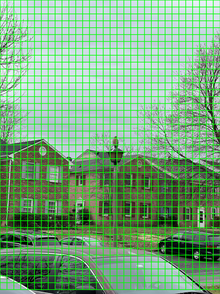
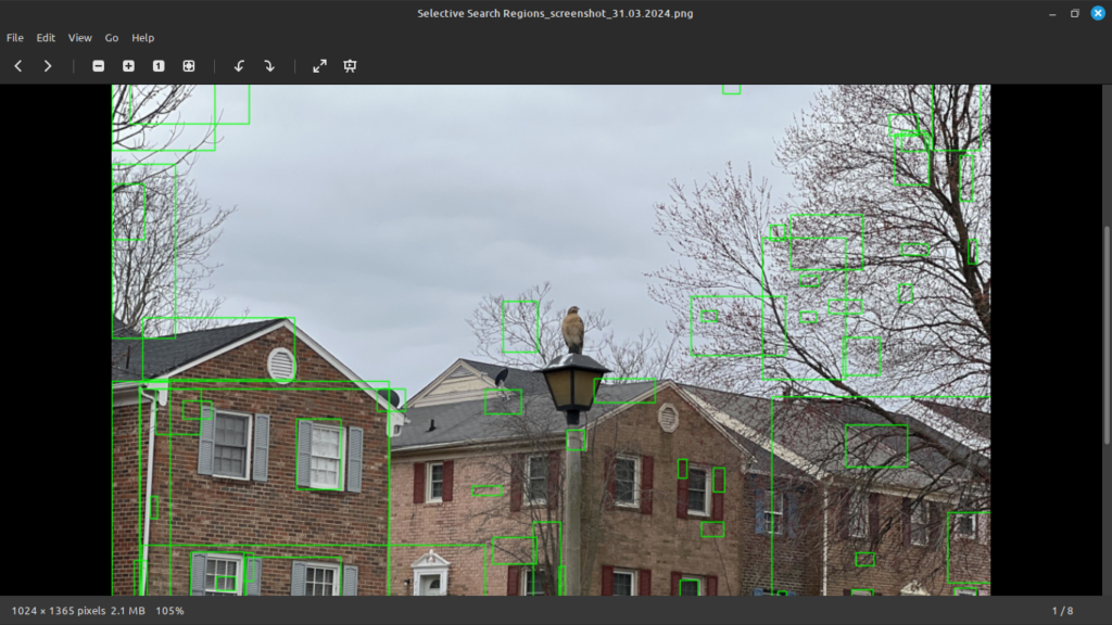
However, selective search is not always perfect.  Below is an example where I ran OpenCV 4’s selective search against an image of mine.  It generated 9,020 proposed areas to search.  I zoomed in to show it did not even show the hawk as a region of interest.

Selective search output run against an image with a hawk.

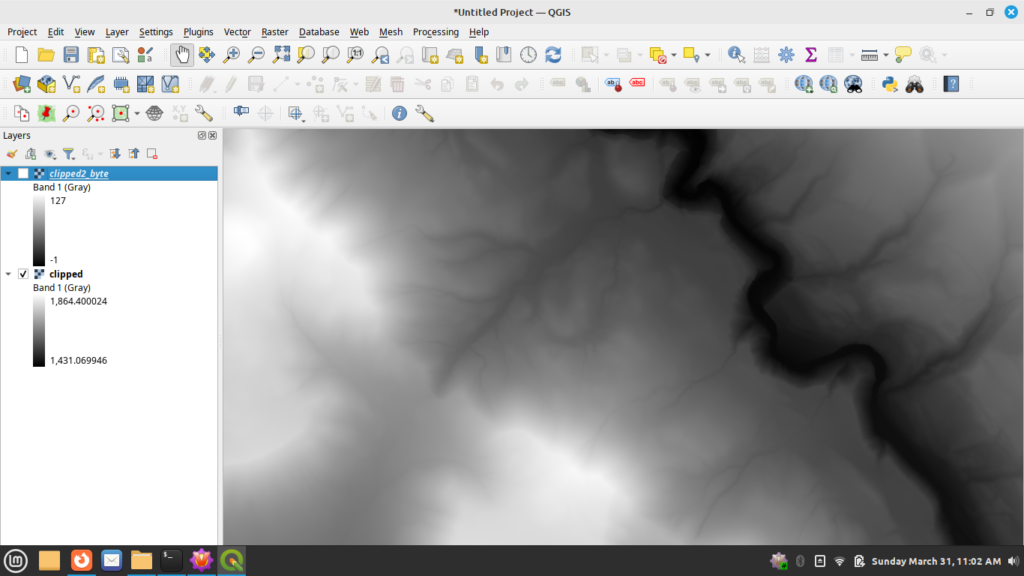
Here’s a clipped version of the input dataset when viewed in QGIS as a 32-bit DEM.  Notice in this case the values range from roughly 1,431 to 1,865.

QGIS with a clip of the original dataset.

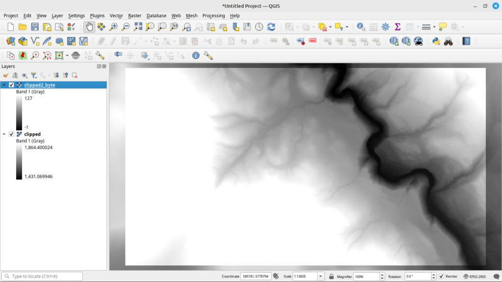
Now here is a version converted to the 8-bit byte format in QGIS.

Same data converted to byte.

As you can see, there is quite a difference between the two files.  And before you ask, int8 just results in a black image no matter how I try to adjust the no-data value.

Tensorflow tf.data Pipeline

So to run this, I set up a Tensorflow tf.data pipeline for processing.  My goal was to be able to turn any of the built-in Tensorflow models into a RCNN.  An interesting artifact of using built-in models, Tensorflow, and OpenCV was that the input data actually had to be converted into RGB format.  Yes, this means a 32-bit grayscale image had to become a 32-bit RGB image, which of course greatly increased the memory requirements.  Here’s a code snippet that shows how to use Rasterio, PIL, and numpy to take an input image and convert it so it’s compatible with the built-in Tensorflow models:

def load_and_preprocess_32bit_image(image_bytes: tensorflow.string) -> numpy.ndarray:
    """Helper function to preprocess 32-bit TIFF image
    Args:
       image_bytes (tensorflow.string): Input image bytes
    Returns:
        numpy.ndarray: decoded image
    """

    with rasterio.io.MemoryFile(image_bytes) as memfile:
        with memfile.open() as dataset:
            image = dataset.read()
    
    image = Image.fromarray(image.squeeze().astype('uint32')).convert('RGB')
    image = numpy.array(image)  # Convert to NumPy array
    image = tensorflow.image.resize(image, local_config.IMAGE_SIZE)

    return image

This function takes the 32-bit DEM, loads it, converts it to a 32-bit RGB image, and then converts it to a format that Tensorflow can work with.  

You can then create a function that can use this as part of a tf.data pipeline by defining a function such as this:


def load_and_preprocess_image_train(image_path, label, in_preprocess_input,
                                    is_32bit=False):
    """ Define a function to load, preprocess, and augment the images
    Args:
        image_path (_type_): Path to the input image
        label (_type_): label of the image
        in_reprocess_input: Function from keras to call to preprocess the input
        is_32bit (bool, optional): Is the image a 32 bit greyscale. Defaults to 
                                   False.

    Returns:
     _type_: Pre-processed image and label
    """

    image = tensorflow.io.read_file(image_path)

    if is_32bit:
        image = tensorflow.numpy_function(load_and_preprocess_32bit_image, 
                                          [image],
                                          tensorflow.float32)
    else:
        image = tensorflow.image.decode_image(image, 
                                              channels=3,
                                              expand_animations=False)
        image = tensorflow.image.resize(image, local_config.IMAGE_SIZE)
     
    image = augment_image_train(image)  # Apply data augmentation for training
    image = in_preprocess_input(image)

    return image, label

Lastly, this can then be set up as a part of your tf.data pipeline by using code like this:

# Create a tf.data.Dataset for training data
train_dataset = tf.data.Dataset.from_tensor_slices((train_image_paths, train_labels))
train_dataset = 
    train_dataset.map(lambda path, label:
        image_utilities.load_and_preprocess_image_train(path,
                                                        label,
                                                        preprocess_input,
                                             is_32bit=local_config.USE_TIF,
                                             num_parallel_calls=tf.data.AUTOTUNE)

(Yeah trying to format code on a page in WordPress doesn’t always work so well)

Note I plan on making all of the code public once I make sure the client is cool with that since I was already working on it before taking on their project.  In the meantime, sorry for being a little bit vague.

Training a Model to be a RCNN

Once you have your pipeline set up, it is time to load the built-in model.  In this case I used Xception from Tensorflow and used the pre-trained model to do transfer learning by the standard omit the top layer, freeze the previous layers, then add a new layer on top that learns from the input.

# Load the model without pre-trained weights
base_model = Xception(weights=local_config.PRETRAINED_MODEL, 
                      include_top=False, 
                      input_shape=local_config.IMAGE_SHAPE,
                      classes=num_classes, input_tensor=input_tensor)

# Freeze the base model layers if we're using a pretrained model

if local_config.PRETRAINED_MODEL is not None:
     for layer in base_model.layers:
         layer.trainable = False

# Add a global average pooling layer
x = base_model.output
x = GlobalAveragePooling2D()(x)

# Create the model
predictions = Dense(num_classes, activation='softmax')(x)
model = Model(inputs=base_model.input, outputs=predictions)

In this case, I used Adam as the optimizer as it performed better than something like the stock SGD and I added in two model callbacks.  The first saves the model to disk every time the validation accuracy goes up, and the second stops processing if the accuracy hasn’t improved over a preset number of epochs.  These are actually built-in to Keras and can be set up as follows:

# construct the callback to save only the *best* model to disk based on 
# the validation loss
model_checkpoint = ModelCheckpoint(args["weights"], 
                                   monitor="val_accuracy", 
                                   mode="max", 
                                   save_best_only=True,
                                   verbose=1)

# Add in an early stopping checkpoint so we don't waste our time
early_stop_checkpoint = EarlyStopping(monitor="val_accuracy",
                                      patience=local_config.EPOCHS_EXIT,
                                      restore_best_weights=True)

You can then add them to a list with

model_callbacks = [model_checkpoint, early_stop_checkpoint]

And then pass that into the model.fit function.

After all of this, it was a matter of running the model.  As you can imagine, training took several hours.  Since this has gotten a bit long, I think I’ll go into how I did the detection stages next time.

Applying Deep Learning and Computer Vision to LiDAR Part1: File Sizes

Introduction

I recently had an interesting project where a client wanted to see if certain geographic features could be found by using deep learning on LiDAR converted to GeoTIFF format.  I had already been working on some code to allow me to use any of the Tensorflow built-in models as R-CNNs, so this seemed like the perfect opportunity to try this.  This effort wasn’t without issues, and I thought I would detail them here in case anyone else is interested.  File sizes, lack of training data, and a video card with an add-on fan that sounded like a jet engine turned out to be interesting problems for the project.

I decided to split this up into multiple posts.  Here in Part 1, I will be covering the implications of doing deep learning and computer vision on LiDAR where file sizes can range in the hundreds of gigabytes for imagery.

What is LiDAR?

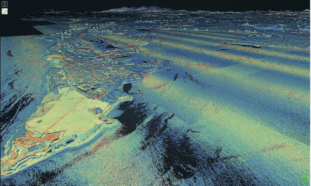
Example LiDAR point cloud courtesy the United States Geological Survey

LiDAR is a technology that uses laser beams to measure distances and movements in an environment. The word LiDAR comes from Light Detection And Ranging, and it works by sending out short pulses of light and measuring the time it takes for them to bounce back from objects or surfaces. You may have even seen it used on your favorite television show, where people will fly a drone to perform a scan of a particular area.  LiDAR can create high-resolution maps of various terrains, such as forests, oceans, or cities. LiDAR is widely used in applications such as surveying, archaeology, geology, forestry, atmospheric physics, and autonomous driving. 

Archaeologists have made a lot of recent discoveries using LiDAR.  In Central and South America, lost temples and other structures from ancient civilizations such as the Aztecs and the Inca have been found in heavily forested areas.  Drone-based LiDAR can be used to find outlines of hard-to-see foundations where old buildings used to stand.

LiDAR scans are typically stored in a point-cloud format, usually LAS or LAZ or other proprietary and unmentionable formats.  These point clouds can be processed in different ways.  It is common to process them to extract the ground level, tree top level, or building outlines.  This is convenient as these points can be processed for different uses, but not so convenient for visualization.

LiDAR converted to a GeoTIFF DEM

These data are commonly converted into GeoTIFF format, a raster file format, so that they can be used in a GIS.  In this form, they are commonly used as high-resolution digital elevation format (DEM) files.  These files can then be used to perform analysis tasks such as terrain modeling, hydrological modeling, and others.

File Sizes

Conversion to GeoTIFF might result in smaller file sizes and can be easier to process in a GIS, but the files can still be very large.  For this project, the LiDAR file was one hundred and three gigabytes. It was stored as a 32-bit grayscale file so that the elevations of each point on the ground could be stored at a high resolution.  This is still an extremely large file, and not able to be fully loaded into memory for deep learning processing unless a very high-end computer was used (spoiler: I do not have a terabyte of RAM on my home computer).

Using CUDA on a GPU became interesting.  I have a 24 gigabyte used Tesla P40 that I got for cheap off eBay.  Deep learning models can require large amounts of memory that can quickly overwhelm a GPU.  Things like data augmentation, where training images are slightly manipulated on the CPU to provide more samples to help with generalization, take up main memory.  The additional size of the 32-bit dataset and training samples led to more memory being taken up than normal.

Deep learning models tend to require training data to be processed in batches.  These batches are small sets of the input data that are processed during one iteration of training.  It’s also more efficient for algorithms such as stochastic gradient descent to work on batches of data instead of the entire dataset during each iteration.  The sheer size of the training data samples meant that each batch took up a large amount of memory.

Finally, it was impossible to run a detection on the entire LiDAR image at one time.  The image had to be broken up into chunks that could be loaded into memory and run in a decent amount of time.  I made a random choice of cutting the image into an 8×8 grid, resulting in sixty-four images.  I wanted to be able to break up the processing so I could run it and combine the results at the end.  At the time, I had not yet water-cooled my Tesla, so the cooling fan I had attached to it sounded like a jet engine while running.  Breaking it into chunks meant that I could process things during the day and then stop at night when I wanted to sleep.  Believe me, working on other projects during the day while listening to that fan probably made me twitch a bit more than normal.

Conclusion

So that’s it for Part 1. I hope I’ve touched on some of the issues that I came across while trying to processing LiDAR with deep learning and computer vision algorithms. In Part 2 I’ll discuss gathering training data (or the lack of available training data).

Some Thoughts on Creating Machine Learning Data Sets

My whole professional career (26 years now!) has been in slinging data around. Be it writing production systems for the government or making deep learning pipelines, I have made a living out of manipulating data. I have always taken pains to make sure what I do is correct and am proud of how obsessive I am about putting things together.

Lately I have been back to doing deep learning and computer vision work and have been looking at some of the open datasets that are out there for satellite imagery. Part of this work has involved trying to combine datasets to train models for object classification from various satellite imagery providers.

One thing I have noticed is that it is still hard to make a good deep learning dataset. We are only human, and we miss things sometimes. It is easy to misclassify things or accidentally include images that might not be a good candidate. Even ImageNet, one of the biggest computer vision and deep learning datasets out there, has been found to contain errors in the training data.

This got me thinking about putting together datasets and what “rules of thumb” I would use for doing so. As there do not seem to be as many articles out there about making datasets versus using them, I thought I would add my two cents on making a good machine learning dataset. This is by no means a criticism about the freely-available datasets out there now. In fact, we should all be thankful so many people are putting them out there, and I hope to add to these soon! So, in no particular order, here we go.

Limit the Number of Object Classes

One thing I have noticed is many datasets try to break out their object classes into too fine of detail. This looks to be especially true for satellite datasets. For example, one popular dataset breaks aircraft down into multiple classes ranging from propeller to trainer to jet aircraft. One problem with this approach is that it becomes easy to pick the wrong category while classifying them. Jet trainers are out there. Should that go into the jet category, or the trainer category? There are commercial propeller aircraft out there. What do we do with them?

It is one thing if you are purposely trying to differentiate different types of aircraft from satellite imagery. Even then, however, I would guess that a neural network would learn mostly the same features for each object class, and you would end up getting the aircraft category correct but have numerous misclassifications for the type. It will also be a lot easier to accidentally mislabel things from imagery while you are building the dataset. Now this is different if you are working with imagery to which only certain types of three letter agencies have access. But, most of us have to make due with the types of imagery that are freely available.

Verify Every Dataset Before Use

We all get into a hurry. We have deadlines, our projects are usually underfunded, and we spend large amounts of time putting out fires. It is still vitally important to not blindly use a dataset to train your model! Consider the below image. In one public domain dataset out there, around eight of these images are all labeled as boats.

Image of a car labeled as a boat.

This is a classical example of “we’re only human.” I would wager that a lot of datasets contain errors such as this. It is not that anyone is trying to purposely mislead you. It just happens sometimes. This is why it is essential to go through your dataset no matter how boring it might be. Labeling is a tough job, and there is probably a room in Hell that tortures people by making them label things all day and night. Again, everyone makes mistakes.

Clean up Your Datasets

Some datasets out there are derived from Google Earth. It is a source of high quality imagery and for now the terms seem to not require your firstborn or an oath of loyalty. The problem comes when you include things like the image below in your training set.

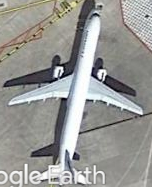
Here you can see that someone used an aircraft that had the Google Earth watermark superimposed on top of it. If you only have one or two, it likely will not be an issue. However, if you have a lot of things like this, then your network could learn features from the text and start to expect imagery to have this in it. This is an example of where you should practice due diligence in cleaning up your data before putting it into a machine learning dataset.

Avoid Clusters (Unless Looking for Them)

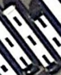
When extracting objects from Google Earth, you might come across something you consider a gold mine. Say you are extracting and labeling cars from imagery, and you come across a full parking lot. This seems like an easy way to suddenly add a lot of training data, and you might end up with a lot of images such as the one below.

In a dataset I recently worked with, there were several object classes that had a lot of images of the same types of objects right next to each other. If you do this, keep in mind that there could be some side effects from having a lot of clusters in your dataset.

  • It could (possibly) be helpful because your object class can present different views if they are present in a cluster. In the above, you can see the top of one bus and the back of another right beside it. This can aid in learning different features for that class.
  • A negative is that if you have a lot of clusters of objects in your training data, your classifier might lean towards detecting objects in groups instead of individual objects. If you are specifically looking for clusters then this is OK. If you want to search for individual ones, then it could hurt your accuracy.
  • The complexity of your training data could increase and lead to slow-downs during the training process by having more features present for each example object than would be present ordinarily.

In general, it is OK to have some clusters of objects in your data. Just be mindful that if you are looking for individual objects, you should try not to have a lot of clusters in your training data.

Avoid Duplicate Objects

This is true for objects in the same class or between object classes. If you have a lot of duplicates, you can run the risk of over-fitting during training. Problems can also arise if you, say, have a car in both a car object class and in a truck class. In this case you can end up with false detections because you accidentally matched the same features in multiple classes.

Pick Representative Training Data

If you are trying to train a model to detect objects from overhead imagery, you would not want to use a training set of pictures people have taken from their cellular phones. Similarly, if you want to predict someone’s mood from a high resolution camera, you would not want to train using fuzzy webcam images. This is stressed in numerous deep learning texts out there, but it is important to repeat. Check if the data you are using for training matches the data you intend to be running your model on. Fitness for use is important.

Invariance

The last thing I want to discuss here is what I feel is one of the most important aspects of deep learning: invariance. Convolutional neural networks are NOT invariant to scale and rotation. They can detect translations, but you do not get scale or rotational invariance by default. You have to provide this using data augmentation during your training phase.

Consider a dataset of numbers that you are using to train a model. This dataset will likely have the numbers written as you would expect them to be: straight up and down. If you train a model on this, it will detect numbers that match a vertical orientation, but accuracy will go down for anything that is off the vertical axis.

Frameworks like Keras make this easy by providing classes or functions that can randomly rotate, shear, or scale images during training before they are input into the network. This helps the classifier learn features in different orientations, something that is important for classifying overhead imagery.

Conclusion

In summary, these are just some general guidelines I use when I am putting together a dataset. I do not always get everything right, and neither will you. Get multiple eyes looking at your dataset and take your time. Labeling is a laborious, and if your attention drifts it is easy to get wrong. The better quality your training data, the better your model will perform.

Using Free Geospatial Tools and Data Part 2: Last of the History Lesson I Promise

As GPS became more popular, another problem came about. Map updates for these units were expensive. They were in proprietary formats and could only be used from a specific vendor for their units. Many units could not be updated at all. Even better, in some cases individual units could not share the same update. The updates were slow to incorporate all new areas. At one point, a popular GPS maker only employed a hand full of cartographers who were responsible for the entire world. As you can imagine, they could only do so much at any given time.

Some enterprising souls decided they wanted to try to convert their expensive data from their proprietary GIS packages and put them on their GPSs. After some reverse engineering they actually managed to get data into a format so they could put maps on their GPS units. Even then the GIS data sets were not current for everywhere as the vendors focused on popular areas.

This approach had a few problems. First, there were not that many people who had the skills and software available to do the GPS reverse engineering and convert the vendor data sets to use with them. The commercial GIS data were not necessarily any better than the GPS data in terms of being up to date. Plus, everything was proprietary. The GPS and GIS data were owned by vendors who would go after people if they even thought about making data available for free to anyone who had not bought a license. So even if you had access to the GIS data and tools, you could only update your own GPS and not post the files online for people to download. And you were likely violating some license agreement even if you only used it for yourself.

If fact, the vendors were very aggressive about protecting their data and took action against anyone who violated their copyright. Early web map companies would introduce errors into their data sets in an attempt to watermark them so they would know when someone was illegally using them. This was before the days of widespread in-car GPS units and Google or NAVTEQ cars driving around recording roads with GPS precision and accuracy. With closed software and data, no one really had to worry about accuracy for the casual user.

Open Source Comes to the Table

The frustrations with proprietary vendors and data sets started a small cottage industry of developers who wanted to give everyone access to the same types of tools that the commercial vendors had. In the commercial GIS space there were only one or two real sellers of GIS software. This monopoly led to stagnant development and large monolithic software programs. These Open Source developers wanted to write new tools that everyone could use to manipulate what free data was out there. They wrote libraries such as GDAL, libgeotiff, and others to provide access to the various file formats. The tools followed to allow users to do simple manipulations of geospatial data.

Now that people had tools, they wanted data to work on. Data at this time was scarce, mainly reposted USGS Digital Raster Graphics (scanned paper maps) and Digital Orthophotos (aerial photographs) in the raster data space. The US Census made their TIGER vector map data (think roads) available for download, but early on it had issues with spatial accuracy and was hard to work with unless the user spent time converting it to work in their GIS. The USGS also had some vector data for hydrography and transportation data but was also somewhat difficult to use due to the formats in which it was distributed.

People at this time had been doing various things with GPS units and early GIS tools to make data available. Some people posted GPS tracks of trails for others to go hiking on. Geocaching had caught on in a big way and introduced a lot of people to the convenience of a GPS. Moving map display GPS units allowed people to navigate roads without need for a paper map. More and more people began wanting up to date data for their devices, and they did not want to pay the expensive prices the commercial vendors wanted.

The explosion in GPS use and availability of Open Source tools to use it led to outcries of people who wanted more data so they could keep their GPS units up to date or just play with photos of their neighborhoods. Technology had evolved to the point where computers could more easily manipulate the large raster data sets that were out there. Eventually governments began to make more data available to the tax payers who felt they paid for it once so should not pay again to download it. The USGS made DRGs and DOQs available for free. The TIGER vector data got a lot more accurate and was updated on a much more regular basis. But still, a lot of the data was not current or up to date since there was only so much money spent by governments on mapping programs.

Along comes the OpenStreetMap (OSM) project in 2004 with the goal of creating a free base map of the world. OSM came out in the early years of the social media craze and provided a collaborative platform so people could add mapping data through either GPS traces or by volunteering their time to vectorize satellite photos. Suddenly, people all over the world could contribute to creating free maps of their areas and use the data however they wanted to use them. Combined with more and more governments providing their data free to download, we came to the modern era where we have more GIS data available than ever before.

Where are we Now?

To be superfluous, we’re now in a golden age of Open Source GIS tools and open data. The very capable QGIS application has recently hit version 2.0. OpenStreetMap continues to grow and is up to a compressed 30 gigabyte file with high-resolution user-contributed data under an open license. Toolkits and libraries such as GDAL power many Open Source and even some commercial applications. Many cars now come with GPS units built-into the dash. Cell phones with 3G+ data connections and mapping apps from Google, Apple, and others have caused traditional GPS companies such as Garmin to scramble to determine their future relevance. Anyone can now take Open Source tools and convert open data to update maps in their GPSs. Web map services using open standards make even more data available to web browsers and other applications. Times have gone from a scarcity of geospatial data to so much that management and discovery of it has become difficult due to the volume and number of providers.

Next time we’ll take a look at the Open Source tools of the trade that anyone can download and use.

Using Free Geospatial Tools and Data Part 1: Introduction and a History Lesson

This kicks off a series of posts about GIS tools and data. I’ve wanted to do something like this for a while now, but am finally forcing myself to do more writing to get back into the habit. So to start off, I’d like to go through a brief history lesson to discuss where GIS was and where it is today. I’ve had a long history in the GIS field, spending most of my professional career working for a government mapping agency where I wrote production systems and then transitioned into a research and development mode. So on to Part 1.

In days of old (OK, only around a decade or three ago), getting into the geospatial field could be a costly endeavor. Most data were locked up in proprietary vaults and you had to pay for access to them, if you could get access at all. The world had just started to transition from paper maps and traditional cartography to applying technology to mapping tasks. With the less advanced technology of the day, transcribing paper maps into a digital representation was a labor-intensive task and required many hours of work. In many cases, creating vector data involved someone drawing vectors on top of an on-screen image of a paper map (which sadly, is still one of the main methods in use today!).

There was also a lot of confusion in the early days about how to do digital mapping in the first place. Most of the people involved came from paper mapping and had spent decades learning how things worked in a physical world. The move to digital changed things. Accuracy in the paper world was no longer sufficient in digital, as what looked like it lined up on paper actually didn’t line up in digital. You could zoom in with a computer and see how far things actually were from lining up. There was a lot of resistance in the early years as mappers did not think using computers was “real” cartography.

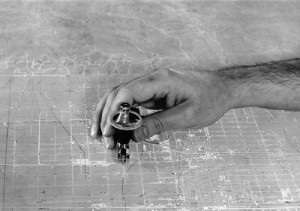
As an example, consider how paper maps were printed. They used multiple Mylar plates that contained various parts of the map. When the map was printed, the plates would be inked and roll against the paper to lay down the layers (colors) of the map. These plates were aligned by the use of stud holes that were cut into the Mylar so they could be positioned correctly during the printing process. When these plates were scanned in and referenced, they did not line up. In the analog world, a gap of a millimeter or so would not really show up on the paper map. In digital, however, that gap will stand out like a sore thumb when the digital map separates are combined in a GIS.


Cartographer scribing a map separate Credit: U.S. Geological Survey Department of the Interior/USGS U.S. Geological Survey.

Cartographer scribing a map separate
Credit: U.S. Geological Survey
Department of the Interior

GIS tools themselves were expensive and were mainly only available from two vendors. Additionally, these tools were really only available on Windows and proprietary UNIX platforms such as Solaris and IRIX. Using them was difficult and required users to have an in-depth understanding of geospatial data and how to use the tools. Many people had to take week long vendor classes before they could use them. And of course, most of the tools had to be run from the command line.

Then things began to change. GPS was opened up to the public and for the first time mapping became dynamic for the non-GIS user. As GPS advanced, they became equipped with moving map displays so people could actually see where they were on a map and could see what was around them.

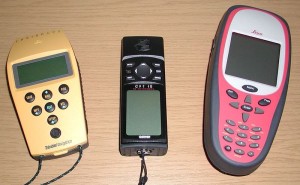
Early GPS, however, also suffered the same issues as early GIS systems. In the beginning they were bulky and only gave you your latitude and longitude on a digital display. This was OK for some people, as they could look at a paper map to reference where they were. They were expensive and only came from a handful of vendors. These early units had accuracy issues, the major being the intentional inaccuracy mandated by the US government who were afraid they could be used against America. They were very dependent on line of sight and took a while to get a general lock (which then meant they were accurate to the tens of feet instead of a foot or two).


Various GPS Receivers Credit: Wikipedia Photographer: Stefan Kühn

Various GPS Receivers
Credit: Wikipedia
Photographer: Stefan Kühn


GPS and GIS technologies began to evolve. GIS software got better and became more user friendly, making use of GUI technologies of the day. GPS technology evolved and became faster and smaller so that people could use hand held units to venture into the outdoors. GIS professionals began to try to hook up their software systems to a GPS so they could use their data with real-time measurements. Companies then got the bright idea to sell software so that you could hook a GPS to your laptop and then watch your location in real time on the screen. It was clunky and hard to use, but was the direct ancestor of every system we take for granted today.

Next time I’ll discuss the rise of Open Source GIS tools and data.