My first professional job during and after college was working at the US Geological Survey as a software engineer and researcher. My job required me to learn about GIS and cartography, as I would do things from writing production systems to researching distributed processing. It gave me an appreciation of cartography and of geospatial data. I especially liked topographic maps as they showed features such as caves and other interesting items on the landscape.

Recently, I had a reason to go back and recreate my mosaics of some Historic USGS Topomaps. I had originally put them into a PostGIS raster database, but over time realized that tools like QGIS and PostGIS raster can be extremely touchy when used together. Even after multiple iterations of trying out various overview levels and constraints, I still had issues with QGIS crashing or performing very slowly. I thought I would share my workflow in taking these maps, mosaicing them, and finally optimizing them for loading into a GIS application such as QGIS.  Note that I use Linux and leave how to install the prerequisite software as an exercise for the reader.

As a refresher, the USGS has been scanning in old topographic maps and has made them freely available in GeoPDF format here. These maps are available at various scales and go back to the late 1800s. Looking at them shows the progression of the early days of USGS map making to the more modern maps that served as the basis of the USGS DRG program. As some of these maps are over one-hundred years old, the quality of the maps in the GeoPDF files can vary widely. Some can be hard to make out due to the yellowing of the paper, while others have tears and pieces missing.

Historically, the topographic maps were printed using multiple techniques from offset lithographic printing to Mylar separates. People used to etch these separates over light tables back in the map factory days. Each separate would represent certain parts of the map, such as the black features, green features, and so on. While at the USGS, many of my coworkers still had their old tool kits they used before moving to digital. You can find a PDF here that talks about the separates and how they were printed. This method of printing will actually be important later on in this series when I describe why some maps look a certain way.

Process

There are a few different ways to start out downloading USGS historic maps. My preferred method is to start at the USGS Historic Topomaps site.

USGS Historic Maps Search

It is not quite as fancy a web interface as the others, but it makes it easier to load the search results into Pandas later to filter and download. For my case, I was working on the state of Virginia, so I selected Virginia with a scale of 250,000 and Historical in the Map Type option. I purposely left Map Name empty and will demonstrate why later.

Topo Map Search

Once you click submit, you will see your list of results. They are presented in a grid view with metadata about each map that fits the search criteria. In this example case, there are eighty-nine results for 250K scale historic maps. The reason I selected this version of the search is that you can download the search results in a CSV format by clicking in the upper-right corner of the grid.

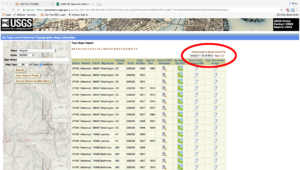
Topo Map Search Results

After clicking Download to Excel (csv) File, your browser will download a file called topomaps.csv. You can open it and see that there is quite a bit of metadata about each map.

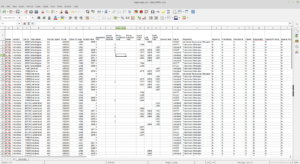
Topo Map CSV Results

If you scroll to the right, you will find the column we are interested in called Download GeoPDF. This column contains the download URL for each file in the search results.

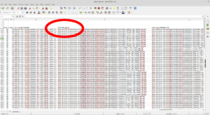
Highlighted CSV Column

For the next step, I rely on Pandas. If you have not heard of it, Pandas is an awesome Python data-analysis library that, among a long list of features, lets you load and manipulate a CSV easily. I usually load it using ipython using the commands in bold below.

bmaddox@sdf1:/mnt/filestore/temp/blog$ ipython3
Python 3.6.6 (default, Sep 12 2018, 18:26:19) 
Type "copyright", "credits" or "license" for more information.

IPython 5.5.0 -- An enhanced Interactive Python.
?         -> Introduction and overview of IPython's features.
%quickref -> Quick reference.
help      -> Python's own help system.
object?   -> Details about 'object', use 'object??' for extra details.

In [1]: import pandas as pd

In [2]: csv = pd.read_csv("topomaps.csv")

In [3]: csv
Out[3]: 
   Series     Version  Cell ID     ...      Scan ID GDA Item ID  Create Date
0    HTMC  Historical    69087     ...       255916     5389860   08/31/2011
1    HTMC  Historical    69087     ...       257785     5389864   08/31/2011
2    HTMC  Historical    69087     ...       257786     5389866   08/31/2011
3    HTMC  Historical    69087     ...       707671     5389876   08/31/2011
4    HTMC  Historical    69087     ...       257791     5389874   08/31/2011
5    HTMC  Historical    69087     ...       257790     5389872   08/31/2011
6    HTMC  Historical    69087     ...       257789     5389870   08/31/2011
7    HTMC  Historical    69087     ...       257787     5389868   08/31/2011
..    ...         ...      ...     ...          ...         ...          ...
81   HTMC  Historical    74983     ...       189262     5304224   08/08/2011
82   HTMC  Historical    74983     ...       189260     5304222   08/08/2011
83   HTMC  Historical    74983     ...       707552     5638435   04/23/2012
84   HTMC  Historical    74983     ...       707551     5638433   04/23/2012
85   HTMC  Historical    68682     ...       254032     5416182   09/06/2011
86   HTMC  Historical    68682     ...       254033     5416184   09/06/2011
87   HTMC  Historical    68682     ...       701712     5416186   09/06/2011
88   HTMC  Historical    68682     ...       701713     5416188   09/06/2011

[89 rows x 56 columns]

In [4]:

As you can see from the above, Pandas loads the CSV in memory along with the column names from the CSV header.

In [6]: csv.columns
Out[6]: 
Index(['Series', 'Version', 'Cell ID', 'Map Name', 'Primary State', 'Scale',
       'Date On Map', 'Imprint Year', 'Woodland Tint', 'Visual Version Number',
       'Photo Inspection Year', 'Photo Revision Year', 'Aerial Photo Year',
       'Edit Year', 'Field Check Year', 'Survey Year', 'Datum', 'Projection',
       'Advance', 'Preliminary', 'Provisional', 'Interim', 'Planimetric',
       'Special Printing', 'Special Map', 'Shaded Relief', 'Orthophoto',
       'Pub USGS', 'Pub Army Corps Eng', 'Pub Army Map', 'Pub Forest Serv',
       'Pub Military Other', 'Pub Reclamation', 'Pub War Dept',
       'Pub Bur Land Mgmt', 'Pub Natl Park Serv', 'Pub Indian Affairs',
       'Pub EPA', 'Pub Tenn Valley Auth', 'Pub US Commerce', 'Keywords',
       'Map Language', 'Scanner Resolution', 'Cell Name', 'Primary State Name',
       'N Lat', 'W Long', 'S Lat', 'E Long', 'Link to HTMC Metadata',
       'Download GeoPDF', 'View FGDC Metadata XML', 'View Thumbnail Image',
       'Scan ID', 'GDA Item ID', 'Create Date'],
      dtype='object')

The column we are interested in is named Download GeoPDF as it contains the URLs to download the files.

In [7]: csv["Download GeoPDF"]
Out[7]: 
0     https://prd-tnm.s3.amazonaws.com/StagedProduct...
1     https://prd-tnm.s3.amazonaws.com/StagedProduct...
2     https://prd-tnm.s3.amazonaws.com/StagedProduct...
3     https://prd-tnm.s3.amazonaws.com/StagedProduct...
4     https://prd-tnm.s3.amazonaws.com/StagedProduct...
5     https://prd-tnm.s3.amazonaws.com/StagedProduct...
6     https://prd-tnm.s3.amazonaws.com/StagedProduct...
7     https://prd-tnm.s3.amazonaws.com/StagedProduct...
                            ...                        
78    https://prd-tnm.s3.amazonaws.com/StagedProduct...
79    https://prd-tnm.s3.amazonaws.com/StagedProduct...
80    https://prd-tnm.s3.amazonaws.com/StagedProduct...
81    https://prd-tnm.s3.amazonaws.com/StagedProduct...
82    https://prd-tnm.s3.amazonaws.com/StagedProduct...
83    https://prd-tnm.s3.amazonaws.com/StagedProduct...
84    https://prd-tnm.s3.amazonaws.com/StagedProduct...
85    https://prd-tnm.s3.amazonaws.com/StagedProduct...
86    https://prd-tnm.s3.amazonaws.com/StagedProduct...
87    https://prd-tnm.s3.amazonaws.com/StagedProduct...
88    https://prd-tnm.s3.amazonaws.com/StagedProduct...
Name: Download GeoPDF, Length: 89, dtype: object

The reason I use Pandas for this step is that it gives me a simple and easy way to extract the URL column to a text file.

In [9]: csv["Download GeoPDF"].to_csv('urls.txt', header=None, index=None)

This gives me a simple text file that has all of the URLs in it.

https://prd-tnm.s3.amazonaws.com/StagedProducts/Maps/HistoricalTopo/PDF/DC/250000/DC_Washington_255916_1989_250000_geo.pdf
https://prd-tnm.s3.amazonaws.com/StagedProducts/Maps/HistoricalTopo/PDF/DC/250000/DC_Washington_257785_1961_250000_geo.pdf
https://prd-tnm.s3.amazonaws.com/StagedProducts/Maps/HistoricalTopo/PDF/DC/250000/DC_Washington_257786_1961_250000_geo.pdf
…
https://prd-tnm.s3.amazonaws.com/StagedProducts/Maps/HistoricalTopo/PDF/WV/250000/WV_Bluefield_254032_1961_250000_geo.pdf
https://prd-tnm.s3.amazonaws.com/StagedProducts/Maps/HistoricalTopo/PDF/WV/250000/WV_Bluefield_254033_1957_250000_geo.pdf
https://prd-tnm.s3.amazonaws.com/StagedProducts/Maps/HistoricalTopo/PDF/WV/250000/WV_Bluefield_701712_1957_250000_geo.pdf
https://prd-tnm.s3.amazonaws.com/StagedProducts/Maps/HistoricalTopo/PDF/WV/250000/WV_Bluefield_701713_1955_250000_geo.pdf

Finally, as there are usually multiple GeoPDF files that cover the same area, I download all of them so that I can go through and pick the best ones for my purposes. I try to find maps that are around the same data, are easily viewable, are not missing sections, and so on. To do this, I use the wget command and use the text file I created as input like so.

bmaddox@sdf1:/mnt/filestore/temp/blog$ wget -i urls.txt 
--2018-09-23 13:00:41--  https://prd-tnm.s3.amazonaws.com/StagedProducts/Maps/HistoricalTopo/PDF/DC/250000/DC_Washington_255916_1989_250000_geo.pdf
Resolving prd-tnm.s3.amazonaws.com (prd-tnm.s3.amazonaws.com)... 52.218.194.10
Connecting to prd-tnm.s3.amazonaws.com (prd-tnm.s3.amazonaws.com)|52.218.194.10|:443... connected.
HTTP request sent, awaiting response... 200 OK
Length: 32062085 (31M) [application/pdf]
Saving to: ‘DC_Washington_255916_1989_250000_geo.pdf’
…
…

Eventually wget will download all the files to the same directory as the text file. In the next installment, I will continue my workflow as I produce mosaic state maps using the historic topographic GeoPDFs.

Since I needed it as part of my job, I finally got around to finishing up the Geonames scripts in my github repository misc_gis_scripts.  In the geonames subdirectory is a bash script called dogeonames.sh.  Create a PostGIS database, edit the bash file, and then run it and it will download and populate your Geonames database for you.

Note that I’m not using the alternatenamesv2 file that they’re distributing now.  I checked with a hex editor and they’re not actually including all fields on each line, and Postgres will not import a file unless each column is there.  I’ll probably add in a Python file to fix it at some point but not now 🙂

I just uploaded all of the 2017 US Census Tiger datasets where I’ve converted them from county-based to state-based ShapeFiles.  You can find them in my GIS Data section.  Let me know of any errors you come across.  Note I haven’t done all of the Census data, just the ones I regularly use.

When I went to import the latest GNIS dataset into my local PostGIS database, I found that it contains the same issues I’ve been reporting for the past few years.   You can find my fixed version of the dataset here.

As a disclaimer, while I used to work there, I no longer have any association with the US Geological Survey or the Board of Geographic Names.

For those interested, here is the list of problems I found and fixed:

ID 45605: Duplicate entry for Parker Canyon, AZ. The coordinates are in Sonora, Mexico.
ID 45606: Duplicate entry for San Antonio Canyon, AZ. The coordinates are in Sonora, Mexico.
ID 45608: Duplicate entry for Silver Creek, AZ. The coordinates are in Sonora, Mexico.
ID 45610: Duplicate entry for Sycamore Canyon, AZ. The coordinates are in Sonora, Mexico.
ID 567773: Duplicate entry for Hovey Hill, ME. The coordinates are in New Brunswick, Canada.
ID 581558: Duplicate entry for Saint John River, ME. The coordinates are in New Brunswick, Canada.
ID 768593: Duplicate entry for Bear Gulch, MT.  The coordinates are in Alberta, Canada.
ID 774267: Duplicate entry for Miners Coulee, MT.  The coordinates are in Alberta, Canada.
ID 774784: Duplicate entry for North Fork Milk River, MT.  The coordinates are in Alberta, Canada.
ID 775339: Duplicate entry for Police Creek, MT.  The coordinates are in Alberta, Canada.
ID 776125: Duplicate entry for Saint Mary River, MT.  The coordinates are in Alberta, Canada.
ID 778142: Duplicate entry for Waterton River, MT.  The coordinates are in Alberta, Canada.
ID 778545: Duplicate entry for Willow Creek, MT.  The coordinates are in Alberta, Canada.
ID 798995: Duplicate entry for Lee Creek, MT.  The coordinates are in Alberta, Canada.
ID 790166: Duplicate entry for Screw Creek, MT.  The coordinates are in British Columbia, Canada.
ID 793276: Duplicate entry for Wigwam River, MT.  The coordinates are in British Columbia, Canada.
ID 1504446: Duplicate entry for Depot Creek, WA.  The coordinates are in British Columbia, Canada.
ID 1515954: Duplicate entry for Arnold Slough, WA.  The coordinates are in British Columbia, Canada.
ID 1515973: Duplicate entry for Ashnola River, WA.  The coordinates are in British Columbia, Canada.
ID 1516047: Duplicate entry for Baker Creek, WA.  The coordinates are in British Columbia, Canada.
ID 1517465: Duplicate entry for Castle Creek, WA.  The coordinates are in British Columbia, Canada.
ID 1517496: Duplicate entry for Cathedral Fork, WA.  The coordinates are in British Columbia, Canada.
ID 1517707: Duplicate entry for Chilliwack River, WA.  The coordinates are in British Columbia, Canada.
ID 1517762: Duplicate entry for Chuchuwanteen Creek, WA.  The coordinates are in British Columbia, Canada.
ID 1519414: Duplicate entry for Ewart Creek, WA. The coordinates are in British Columbia, Canada.
ID 1520446: Duplicate entry for Haig Creek, WA. The coordinates are in British Columbia, Canada.
ID 1520654: Duplicate entry for Heather Creek, WA. The coordinates are in British Columbia, Canada.
ID 1521214: Duplicate entry for International Creek, WA. The coordinates are in British Columbia, Canada.
ID 1523541: Duplicate entry for Myers Creek, WA. The coordinates are in British Columbia, Canada.
ID 1523731: Duplicate entry for North Creek, WA. The coordinates are in British Columbia, Canada.
ID 1524131: Duplicate entry for Pack Creek, WA. The coordinates are in British Columbia, Canada.
ID 1524235: Duplicate entry for Pass Creek, WA. The coordinates are in British Columbia, Canada.
ID 1524303: Duplicate entry for Peeve Creek, WA. The coordinates are in British Columbia, Canada.
ID 1525297: Duplicate entry for Russian Creek, WA. The coordinates are in British Columbia, Canada.
ID 1525320: Duplicate entry for Saar Creek, WA. The coordinates are in British Columbia, Canada.
ID 1527272: Duplicate entry for Togo Creek, WA. The coordinates are in British Columbia, Canada.
ID 1529904: Duplicate entry for McCoy Creek, WA. The coordinates are in British Columbia, Canada.
ID 1529905: Duplicate entry for Liumchen Creek, WA. The coordinates are in British Columbia, Canada.
ID 942345: Duplicate entry for Allen Brook, NY. The coordinates are in Quebec, Canada.
ID 949668: Duplicate entry for English River, NY. The coordinates are in Quebec, Canada.
ID 959094: Duplicate entry for Oak Creek, NY. The coordinates are in Quebec, Canada.
ID 967898: Duplicate entry for Trout River, NY. The coordinates are in Quebec, Canada.
ID 975764: Duplicate entry for Richelieu River, VT. The coordinates are in Quebec, Canada.
ID 1458184: Duplicate entry for Leavit Brook, VT. The coordinates are in Quebec, Canada.
ID 1458967: Duplicate entry for Pike River, VT. The coordinates are in Quebec, Canada.
ID 1028583: Duplicate entry for Cypress Creek, ND. The coordinates are in Manitoba, Canada.
ID 1035871: Duplicate entry for Mowbray Creek, ND. The coordinates are in Manitoba, Canada.
ID 1035887: Duplicate entry for Gimby Creek, ND. The coordinates are in Manitoba, Canada.
ID 1035890: Duplicate entry for Red River of the North, ND. The coordinates are in Manitoba, Canada.
ID 1035895: Duplicate entry for Wakopa Creek, ND. The coordinates are in Manitoba, Canada.
ID 1930555: Duplicate entry for Red River of the North, ND. The coordinates are in Manitoba, Canada.
ID 1035882: Duplicate entry for East Branch Short Creek, ND. The coordinates are in Saskatchewan, Canada.
ID 1782010: Duplicate entry for Manitoulin Basin, MI. The coordinates are in Ontario, Canada

Yes, it’s close to the end of the year…. but I’m currently putting together the Census 2015 Tiger data and will have it uploaded here under the GIS Data page.  Stay tuned.

Here’s the first map I’ve done based on the GeoPDFs from the USGS Historic Map Collection.  I found all of the available maps for Virginia at the 125K scale and the vintages were from 1888 to 1902.  It’s a GeoTIFF that is 484M in size and compressed using LZW lossless compression.

Link to the map.

For this installment, we will look at importing data from OpenStreetMap.org.  As I mentioned in an earlier post, OpenStreetMap is a cloud-sourced GIS dataset with the goal of producing a global dataset that anyone can use.  There are two ways to download this data: you can either use Bittorrent and download the entire planet from http://osm-torrent.torres.voyager.hr/ or download extracts from http://download.geofabrik.de/.  If you do not need the entire planet, I would highly recommend using geofabrik.  It has a fast downlink and they have finally added MD5 checksums so you can verify the integrity of your download.

Go to http://download.geofabrik.de/ and click on North America.  We will be using the .pbf format file so click the link near the top of the page named north-america-latest.osm.pbf.  It is about six gigabytes in size and the MD5sum is listed at the end of the paragraph.  Once the download is done in your browser, you can use the md5sum command under a Linux shell or download one of the many MD5sum clients for windows.  It will look similar to the below example output (it likely will not match exactly as the MD5 value will change as the data is modified.

bmaddox@girls:~/Downloads/geodata$ md5sum north-america-latest.osm.pbf 
d2daa9c7d3ef4dead4a2b5f790523e6d north-america-latest.osm.pbf
bmaddox@girls:~/Downloads/geodata$

Next go back to the main geofabrik site and then click on and download the Central America file.  This will give you Mexico and the other Central American files.  As listed above, once the download is done in your browser, check it with md5sum.  If the values do not match, you will want to redownload and rerun md5sum again until they do.

There are several programs you can use to import OpenStreetMap data into PostGIS.  They mainly differ on what schema they use and how they manipulate the data before it goes in.  For purposes of this post, we will be using the imposm program found at http://imposm.org/docs/imposm/latest/.  If you are on Ubuntu, it should be a simple apt-get install imposm away.  For Windows or other distributions, you can download it directly from the imposm website.  The tutorial on how to import data using imposm can be found here: http://imposm.org/docs/imposm/latest/tutorial.html.

Using imposm is a multi-stage process.  The first stage is to have it read the data and combine the files into several intermediary files.  First create a PostGIS database by running:

createdb -T gistemplate OSM

Now have imposm take the data and convert it into its intermediary files.  To do this, run a similar command to this:

bmaddox@girls:/data/data/geo$ imposm --read --concurrency 2 --proj EPSG:4326 ~/Downloads/geodata/*.pbf
[16:29:15] ## reading /home/bmaddox/Downloads/geodata/central-america-latest.osm.pbf
[16:29:15] coords: 500489k nodes: 10009k ways: 71498k relations: 500k (estimated)
[16:31:27] coords: 21524k nodes: 92k ways: 2464k relations: 5k
[16:31:28] ## reading /home/bmaddox/Downloads/geodata/north-america-latest.osm.pbf
[16:31:28] coords: 500489k nodes: 10009k ways: 71498k relations: 500k (estimated)
[17:40:22] coords: 678992k nodes: 1347k ways: 44469k relations: 229k
[17:40:23] reading took 1 h 11m 7 s
[17:40:23] imposm took 1 h 11m 7 s
bmaddox@girls:/data/data/geo$

Here, I changed to a different drive and can the imposm command to read from the drive where I downloaded the .pbf files.  I did this since reading is a disk intensive process and spitting it between drives helps to speed things up a bit.  Also, I differed from the tutorial as my install of QGIS could not render OpenStreetMap data in its native EPSG:900913 projection with data in the EPSG:4326 coordinate system that my Tiger data was in.  Unless you have an extremely high-end workstation, this will take a while.  Once the process is done, you will have the following files in the output directory:

bmaddox@girls:~/Downloads/geodata/foo$ dir
imposm_coords.cache imposm_nodes.cache imposm_relations.cache imposm_ways.cache

The next step is to take the intermediary files and write them into PostGIS.  Here you can use a wild card to read all of the .pbf files you downloaded.

bmaddox@girls:~/Downloads/geodata/foo$ imposm --write --database OSM --host localhost --user bmaddox --port 5432 --proj EPSG:4326
password for bmaddox at localhost:
[18:20:21] ## dropping/creating tables
[18:20:22] ## writing data
[2014-06-15 18:52:46,074] imposm.multipolygon - WARNING - building relation 1834172 with 8971 ways (10854.8ms) and 8843 rings (2293.0ms) took 426854.5ms
[2014-06-15 19:00:47,635] imposm.multipolygon - WARNING - building relation 2566179 with 4026 ways (4717.3ms) and 3828 rings (1115.6ms) took 89522.6ms
[19:15:20] relations: 244k/244k
[19:15:41] relations: total time 55m 18s for 244095 (73/s)
[00:35:28] ways: 46907k/46907k
[00:35:30] ways: total time 5 h 19m 49s for 46907462 (2444/s)
[00:40:21] nodes: 1437k/1437k
[00:40:22] nodes: total time 4 m 51s for 1437951 (4933/s)
[00:40:22] ## creating generalized tables
[01:44:47] generalizing tables took 1 h 4 m 24s
[01:44:47] ## creating union views
[01:44:48] creating views took 0 s
[01:44:48] ## creating geometry indexes
[02:15:02] creating indexes took 30m 14s
[02:15:02] writing took 7 h 54m 41s
[02:15:02] imposm took 7 h 54m 42s
bmaddox@girls:~/Downloads/geodata/foo$

As you can see from the above output, this took almost eight hours on my home server (quad core AMD with eight gig of RAM).  This command loads all of the data from the intermediate files into PostGIS.  However, we are not done yet.  Looking at the output, all it did was load the data and create indices.  It did not cluster the data or perform any other optimizations.  To do this, run the following imposm command:

bmaddox@girls:~/Downloads/geodata/foo$ imposm --optimize -d OSM --user bmaddox
password for bmaddox at localhost:
[17:18:12] ## optimizing tables
Clustering table osm_new_transport_areas
Clustering table osm_new_mainroads
Clustering table osm_new_buildings
Clustering table osm_new_mainroads_gen1
Clustering table osm_new_mainroads_gen0
Clustering table osm_new_amenities
Clustering table osm_new_waterareas_gen1
Clustering table osm_new_waterareas_gen0
Clustering table osm_new_motorways_gen0
Clustering table osm_new_aeroways
Clustering table osm_new_motorways
Clustering table osm_new_transport_points
Clustering table osm_new_railways_gen0
Clustering table osm_new_railways_gen1
Clustering table osm_new_landusages
Clustering table osm_new_waterways
Clustering table osm_new_railways
Clustering table osm_new_motorways_gen1
Clustering table osm_new_waterareas
Clustering table osm_new_places
Clustering table osm_new_admin
Clustering table osm_new_minorroads
Clustering table osm_new_landusages_gen1
Clustering table osm_new_landusages_gen0
Vacuum analyze
[19:24:38] optimizing took 2 h 6 m 25s
[19:24:38] imposm took 2 h 6 m 26s
bmaddox@girls:~/Downloads/geodata/foo$

On my system it took a couple of hours and clustered all of the tables and then did a vacuum analyze to update the database statistics.

The final step is to have imposm rename the tables to what they will be in “production mode”.  Run the following:

bmaddox@girls:~/Downloads/geodata/foo$ imposm -d OSM --user bmaddox --deploy-production-tables
password for bmaddox at localhost:
[11:00:06] imposm took 1 s
bmaddox@girls:~/Downloads/geodata/foo$

Your data should now be optimized and ready for use.  To test it, refer to an earlier post in this series where I discussed using QGIS and load some of the OSM data into it.

Your OSM database will have the following tables in it:

 List of relations
 Schema | Name | Type | Owner 
--------+----------------------+-------+---------
 public | osm_admin | table | bmaddox
 public | osm_aeroways | table | bmaddox
 public | osm_amenities | table | bmaddox
 public | osm_buildings | table | bmaddox
 public | osm_landusages | table | bmaddox
 public | osm_landusages_gen0 | table | bmaddox
 public | osm_landusages_gen1 | table | bmaddox
 public | osm_mainroads | table | bmaddox
 public | osm_mainroads_gen0 | table | bmaddox
 public | osm_mainroads_gen1 | table | bmaddox
 public | osm_minorroads | table | bmaddox
 public | osm_motorways | table | bmaddox
 public | osm_motorways_gen0 | table | bmaddox
 public | osm_motorways_gen1 | table | bmaddox
 public | osm_places | table | bmaddox
 public | osm_railways | table | bmaddox
 public | osm_railways_gen0 | table | bmaddox
 public | osm_railways_gen1 | table | bmaddox
 public | osm_transport_areas | table | bmaddox
 public | osm_transport_points | table | bmaddox
 public | osm_waterareas | table | bmaddox
 public | osm_waterareas_gen0 | table | bmaddox
 public | osm_waterareas_gen1 | table | bmaddox
 public | osm_waterways | table | bmaddox
 public | spatial_ref_sys | table | bmaddox
(25 rows)

The _gen0 and _gen1 tables are generalized and not as highly detailed as the other tables.  They are good for viewing data over large geographic areas (think nation scale).  With areas that large, it would take a lot of time to render the high resolution data.  Thus the _gen0 and _gen1 tables are simplified versions of the data for use at these resolutions.  You can use QGIS’s scale-dependent rendering to specify these tables and then go to the high-resolution tables upon zooming in.

Go forth and play with the additional free geospatial data you now have in your database 🙂

Updated 23 March 2018: Changed for new size necessary for the cc2 column

It’s been a while since I’ve made a post, so thought I’d keep going with the data series.  This time around I’ll be talking about how to make your own local copy of the NGA Geonames database.  This database is similar to GNIS, but covers the whole globe and also has information on location such as airfields, pipelines, and so on.

First, download the following files from the Geonames website:

• admin1CodesASCII.txt
• admin2Codes.txt
• allCountries.txt
• alternateNamesV2.txt
• countryInfo.txt
• featureCodes_en.txt
• hierarchy.txt
• iso-languagecodes.txt
• timeZones.txt
• userTags.txt

Some of them are zipped, so you’ll need to unzip them into the same directory as the others for ease of use.  Next, create your geonames database by running:

bmaddox@girls:~/Downloads/geodata$ createdb -T gistemplate Geonames

Next, we will create the table for the main points file, which is called allCountries.txt.  Run the following command from the same directory where you have all of the Geonames files:

bmaddox@girls:~/Downloads/geodata$ psql -d Geonames 
psql (9.3.4)
Type "help" for help.
Geonames=#

This will put you into the PostgreSQL command line.  Now create the table to hold the data in the allCountries.txt file:

Geonames=# create table geoname (
geonameid int,
name varchar(200),
asciiname varchar(200),
alternatenames text,
latitude float,
longitude float,
fclass char(1),
fcode varchar(10),
country varchar(2),
cc2 varchar(170),
admin1 varchar(20),
admin2 varchar(80),
admin3 varchar(20),
admin4 varchar(20),
population bigint,
elevation int,
dem int,
timezone varchar(40),
moddate date
);
CREATE TABLE
Geonames=#

Now we will use a built-in PostgreSQL command to load data in the DB.  There are two forms of it, the long way specifies the column names in order on the command line, the other just the file name.  We will be using the short way here:

Geonames=# \copy geoname from allCountries.txt null as '';
Geonames=#

This loads the data, but it is not yet ready to be usable by a GIS.  We will need to create a geometry column for the data and then use the latitude and longitude columns to create a point column in the geometry.

Geonames=# SELECT AddGeometryColumn( 'geoname', 'the_geom', 4326, 'POINT', 2);
 addgeometrycolumn 
------------------------------------------------------
 public.geoname.the_geom SRID:4326 TYPE:POINT DIMS:2 
(1 row)
Geonames=#

This command creates the geometry column, and specifies an EPSG of 4326 (WGS84).  Now we need to insert the latitude and longitudes of the points into this column:

Geonames=# update geoname SET the_geom = ST_PointFromText('POINT(' || longitude || ' ' || latitude || ')', 4326);
UPDATE 8943136
Geonames=#

This will take a while as PostGIS must read each point, convert it into the proper format, and then add it into the geometry column.  Now we need to add a geospatial index on this column to make the queries faster.  Again, it may take a while to run.

Geonames=# create index geoname_the_geom_gist_idx on geoname using gist (the_geom);
CREATE INDEX
Geonames=#

Once this is done, we should optimize this table as I mentioned in a previous post.  We need to analyze the database and then cluster it on the points.

Geonames=# vacuum analyze geoname;
VACUUM
Geonames=# cluster geoname using geoname_the_geom_gist_idx;
CLUSTER
Geonames=# analyze geoname;

There are several auxiliary tables we should now add to the geonames database.  These define the values used in the various columns and can be used in a JOIN statement in a GIS.  I’m going to leave out the vacuum analyze steps but you should perform it on each table below.  The first will be the alternatename table, which holds data from the  alternateNames.txt file.  This file contains a list of other names some of the points are known by and is connected to the geoname table by the geonameId column:

Geonames=# create table alternatename (
alternatenameId int,
geonameid int,
isoLanguage varchar(7),
alternateName varchar(400),
isPreferredName boolean,
isShortName boolean,
isColloquial boolean,
isHistoric boolean
);
CREATE TABLE
Geonames=# \copy alternatename from alternateNames.txt null as '';
Geonames=#

Next we move on to the iso-languagecodes.txt file.  This file contains ISO-638 standard names for all of the countries in the database.

Geonames=# create table "isolanguage" (
 iso_639_3 char(3),
 iso_639_2 char(10),
 iso_639_1 char(3),
 language_name varchar(100)
);
CREATE TABLE
Geonames=# \copy isolanguage from iso-languagecodes.txt null '' delimiter E'\t' csv header
Geonames=#

Next we will create and load the countryInfo.txt file, which contains information about each country such as iso codes, phone number formats, and so on.  First, we need to remove the comment lines from the start of the file to make things easier.  You can either do this with a text editor and delete every line that starts with the # character, or you can run the following command from bash:

bmaddox@girls:~/Downloads/geodata$ egrep -v "^[[:blank:]]*#" countryInfo.txt > countryInfo2.txt

With this done, we can proceed with the import as normal:

Geonames=# create table "countryinfo" ( 
 iso_alpha2 char(2),
 iso_alpha3 char(3),
 iso_numeric integer,
 fips_code varchar(3),
 name varchar(200),
 capital varchar(200),
 areainsqkm double precision,
 population integer,
 continent varchar(2),
 tld varchar(10),
 currencycode varchar(3),
 currencyname varchar(20),
 phone varchar(20),
 postalcode varchar(100),
 postalcoderegex varchar(200),
 languages varchar(200),
 geonameId int,
 neighbors varchar(50),
 equivfipscode varchar(3)
);
CREATE TABLE
Geonames=# \copy countryinfo from countryInfo2.txt null as '';
Geonames=#

Next we do the timeZones.txt file:

Geonames=# create table "timezones" (
countrycode char(2),
TimeZoneId varchar(30),
gmtoffset double precision,
dstoffset double precision,
rawoffset double precision
);
CREATE TABLE
Geonames=# \copy timezones from timeZones.txt null '' delimiter E'\t' csv header
Geonames=#

Next we do the admin1CodesASCII.txt table, which matches ascii names of administrative divisions to their codes:

Geonames=# CREATE TABLE "admin1codesascii" ( 
code CHAR(10), 
name TEXT, 
nameAscii TEXT, 
geonameid int 
); 
CREATE TABLE
Geonames=# \copy admin1codesascii from admin1CodesASCII.txt null as '';
Geonames=#

Now we do the admin2Codes.txt file that maps the admin2code values to their textual entries.

Geonames=# CREATE TABLE "admin2codes" (
 code varchar(30),
 name_local text,
 name text,
 geonameid int
);
CREATE TABLE
Geonames=# \copy admin2codes from admin2Codes.txt null as '';
Geonames=#

Next is featureCodes_en.txt, which maps feature codes to their descriptions:

Geonames=# CREATE TABLE "featurecodes" ( 
code CHAR(7), 
name VARCHAR(200), 
description TEXT 
); 
CREATE TABLE
Geonames=# \copy featurecodes from featureCodes_en.txt null as '';
Geonames=#

Next is the userTags.txt file that contains user-contributed tagging to the points.

Geonames=# create table "usertags" (
geonameid int,
tag varchar(40)
);
CREATE TABLE
Geonames=# \copy usertags from userTags.txt null as '';
Geonames=#

Finally we will handle the hierarchy.txt file, which contains parent-child relationships modeled from the admin1-4 codes.

Geonames=# create table "hierarchy" (
parentId int,
childId int,
type varchar(40)
);
CREATE TABLE
Geonames=# \copy hierarchy from hierarchy.txt null as '';
Geonames=#

You now should have your own complete copy of the Geonames database.  They do publish updates regularly, so you can either recreate the tables or enter in their changes files.  You may also wish to index the type column of allcountries so you can create custom views that only display things like airports, towers, and so on.

The USGS Board on Geographic Names maintains the Geographic Names Information System (GNIS) database.  It is a database of over two million points in the United States.  This database:

contains information about physical and cultural geographic features in the United States and associated areas, both current and historical (not including roads and highways). The database holds the Federally recognized name of each feature and defines the location of the feature by state, county, USGS topographic map, and geographic coordinates.

You can download the 79 megabyte GNIS zip file from here.  You will want to select the NationalFile as it is not broken up into individual states.  Importing GNIS into PostGIS is slightly more complicated as it does not come as a Shapefile, but instead as a 293 megabyte text file once it is unzipped from the  above.  Download the file, unzip it, and open a command window where the unzipped file is.  Note that the last time I did this on Windows, using the command line client was an exercise in pain due to how Windows handles code pages and character types.  On Windows it might be easier to do this inside something like pgadmin.

To import, first create a database inside PostgreSQL using something like the following:

createdb -T gistemplate USGS

Once done, you will want to run

psql -d USGS

to start the PostgreSQL database client.  Now you will want to create the table to hold the data.  To do this, copy and paste this statement into the psql client window:

CREATE TABLE gnis
(
 feature_id integer NOT NULL,
 feature_name character varying,
 feature_class character varying,
 state_alpha character(2),
 state_numeric character(2),
 county_name character varying,
 county_numeric character(3),
 primary_lat_dms character varying,
 prim_long_dms character varying,
 prim_lat_dec real,
 prim_long_dec real,
 source_lat_dms character varying,
 source_long_dms character varying,
 source_lat_dec real,
 source_long_dec real,
 elev_in_m integer,
 elev_in_ft integer,
 map_name character varying,
 date_created date,
 date_edited date
);

Note that I COULD have spent the time figuring out the maximum size of each column, instead of just making them varchars, to save space.  But, again, I’m lazy 🙂

Now to import, you will run the following command.  The .txt files is over two million rows, so it could take a while to import depending on the speed of your system.

 USGS=# \copy gnis from NationalFile_20140204.txt DELIMITER '|' CSV HEADER

If you get a file not found error,run \copy with the full path to the NationalFile.  Depending on when you do this, the file name may be different based on when it was last updated.

We are not done yet.  There is no actual geospatial geometry column in the database.  We will need to create one from the existing columns.  To do this, first we must create a geometry column to hold the geospatial points.

USGS=# SELECT AddGeometryColumn('public', 'gnis', 'geom', 4326, 'POINT', 2);

This command tells PostgreSQL to add a geometry column named geom to the gnis table in the public schema using NAD83.  Now we need to actually populate this column.  We need to take the latitude and longitude columns in the table and convert them into a binary representation that PostGIS uses internally.

USGS=# update public.gnis 
SET geom = ST_PointFromText('POINT(' || prim_long_dec || ' ' || prim_lat_dec || ')', 4326);

Here we have PostgreSQL convert the prim_long_dec and prim_lat_dec columns into a POINT and then to the actual geometry using the ST_PointFromText function inside PostGIS.

Now we need to add a geospatial index on the geom column.  You need an index to use the data in apps such as QGIS as it makes area look-ups much faster.

USGS=# create index gnis_geom_gist_idx on gnis using gist(geom);

Now that we have an index, we need to create our database statistics and cluster it on the geom column.  As I mentioned in a previous post, you will run these commands in order (waiting for each one to complete before running the next):

USGS=# vacuum analyze gnis;
USGS=# cluster gnis using gnis_geom_gist_idx;
USGS=# analyze gnis;

And now we are done.  You have your own local copy of GNIS that you can use in visual GIS tools or from the command line.  There are some fun things you can do with the data, such as the below figure shows where I used QGIS to load all points in GNIS that have my last name in them (my modesty astounds even me 😉

Maddox Places in QGIS

Happy GISing!

Check out my GIS data section here.  I’ve uploaded state-based Shapefiles of the Census ROADS, LINEARWATER, and others.