Stupid LiDAR Tricks Part 1 (Segmentation)

My last few posts have been about applying machine learning to try to extract geographic objects in LiDAR.  I think now I would like to go in another direction and talk about ways to help us find anything in LiDAR.  There is a lot of information in LiDAR, and sometimes it would be nice to have a computer help us to find areas we need to examine.

In this case I’m not necessarily just talking about machine learning.  Instead, I am discussing algorithms that can examine an image and identify areas that have something “interesting” in them.  Basically, trying to perform object detection without necessarily determining the object’s identity.

For the next few posts, I think I’ll talk about:

I have a GitHub repository where I’ll stick code that I’m using for this series.

Selective Search (OpenCV)

This first post will talk about selective search, in this specific case, selective search from OpenCV.  Selective search is a segmentation technique used to identify potential regions in an image that might contain objects. In the context of object detection, it can help to quickly narrow down areas of interest before running more complex algorithms. It performs:

  1. Segmentation of the Image: The first step in selective search is to segment the image into multiple small segments or regions. This is typically done using a graph-based segmentation method. The idea is to group pixels together that have similar attributes such as color, texture, size, and shape.
  2. Hierarchical Grouping: After the initial segmentation, selective search employs a hierarchical grouping strategy to merge these small regions into larger ones. It uses a variety of measures to decide which regions to merge, such as color similarity, texture similarity, size similarity, and shape compatibility between the regions. This process is repeated iteratively, resulting in a hierarchical grouping of regions from small to large.
  3. Generating Region Proposals: From this hierarchy of regions, selective search generates region proposals. These proposals are essentially bounding boxes of areas that might contain objects.
  4. Selecting Between Speed and Quality: Selective search allows for configuration between different modes that trade off between speed and the quality (or thoroughness) of the region proposals. “Fast” mode, for example, might be useful in cases of real-time segmentation in videos.  “Quality” is used when processing speed is less important than accuracy.

Additionally. OpenCV allows you to apply various “strategies” to modify the region merging and proposal process.  These strategies are:

  1. Color Strategy: This strategy uses the similarity in color to merge regions. The color similarity is typically measured using histograms of the regions. Regions with similar colors are more likely to be merged under this strategy. This is useful in images where color is a strong indicator of distinct objects.
  2. Texture Strategy: Texture strategy focuses on the texture of the regions. Textures are usually analyzed using local binary patterns or gradient orientations, and regions with similar texture patterns are merged. This strategy is particularly useful in images where texture provides significant information about the objects, such as in natural scenes.
  3. Size Strategy: The size strategy prioritizes merging smaller regions into bigger ones. The idea is to prevent over-segmentation by reducing the number of very small, likely insignificant regions. This strategy tries to control the sizes of the region proposals, balancing between small regions with no areas of interest to large areas that contain multiple areas of interest.
  4. Fill Strategy: This strategy considers how well a region fits within its bounding box. It merges regions that together can better fill a bounding box, minimizing the amount of empty space. The fill strategy is effective in creating more coherent region proposals, especially for objects that are close to being rectangular or square.

Selective Search in Action

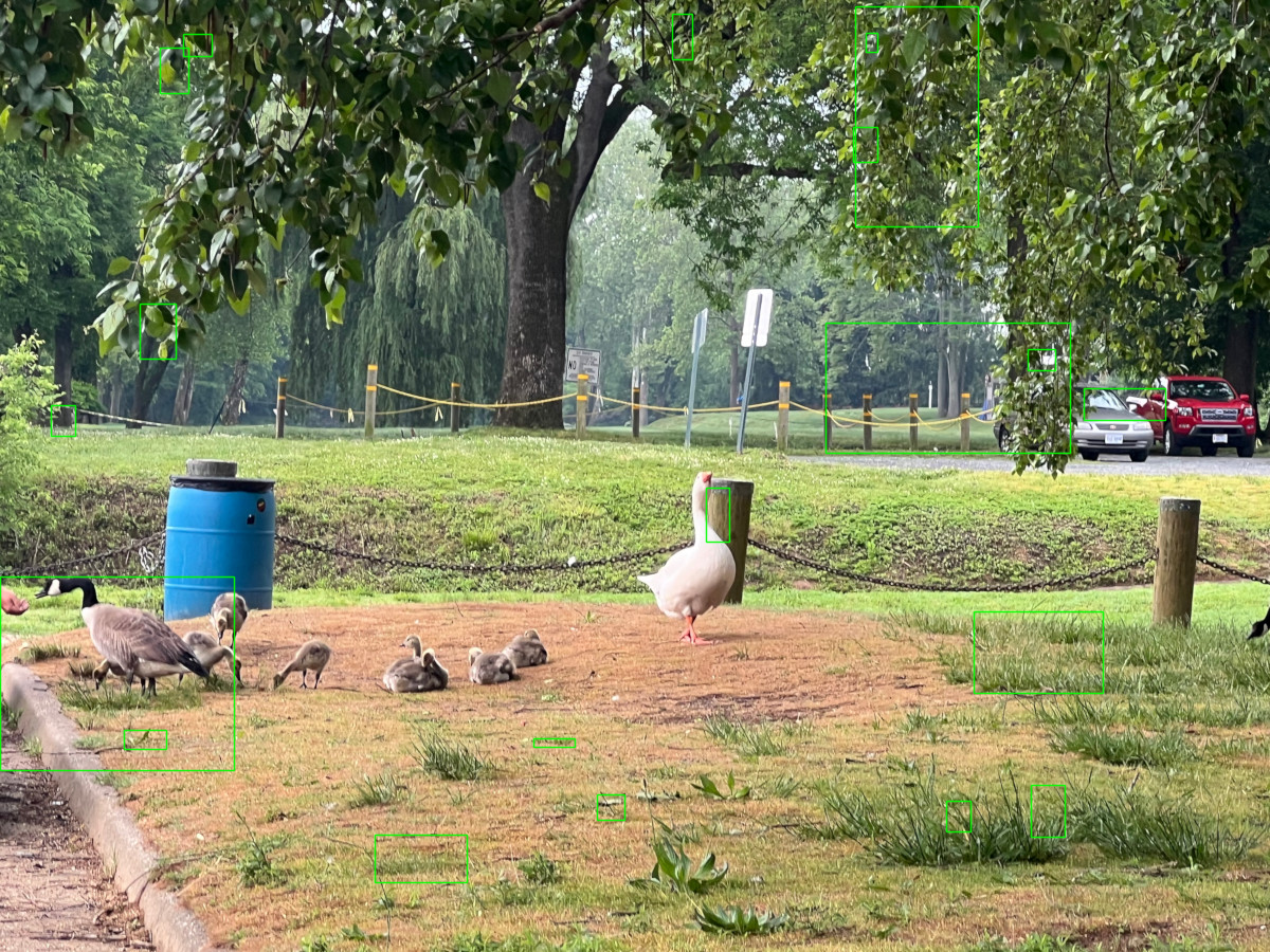
Now let us take a look at how selective search works.  This image is of a local celebrity called Gary the Goose.  To follow along, see the selective_search.py code under the selective_search directory in the above GitHub repository.

Gary the Goose

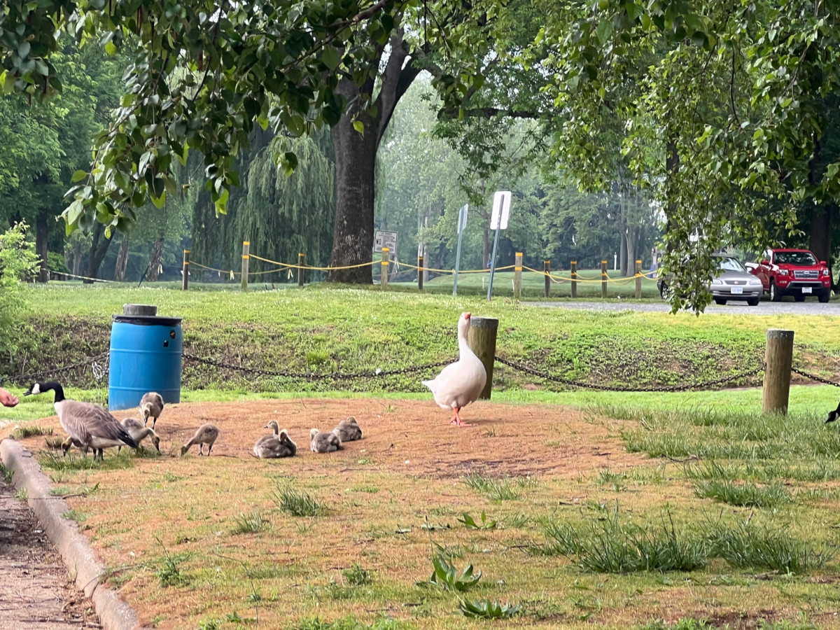
Now let us see how selective search worked on this image:

Selective search on image with all strategies applied.

For this run, selective search was set to quality mode and had all of the strategies applied to it.  As you can see, it found some areas of interest.  It got some of the geese, a street sign, and part of a truck.  But it did not get everything, including the star of the picture.  Now let us try it again, but without applying any of the strategies (comment out line 95).

Default selective search with no strategies applied.

Here we see it did about the same.  Got closer to the large white goose, but still seems to not have picked up a lot in the image.

Selective Search on LiDAR

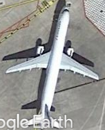
Now let us try it on a small LiDAR segment.  Here is the sample of a townhome neighborhood.

Small LiDAR clip in QGIS

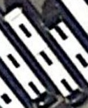
And here is the best result I could get after running selective search:

Selective search run against LiDAR

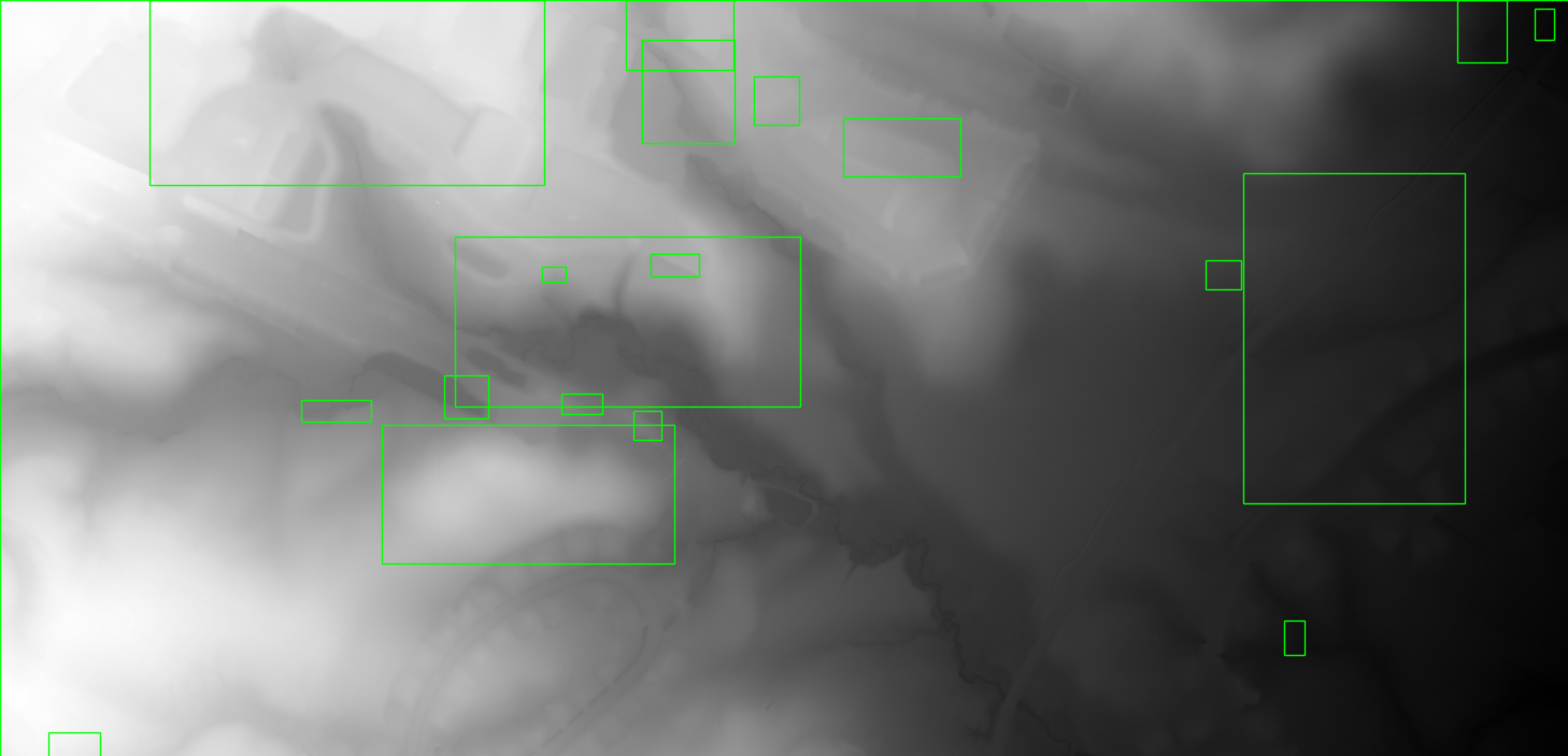
As you can see, it did “ok”.  It identified a few areas, but did not pick up on the houses or the small creeks that run through the neighborhood. 

Selective Search on a Hill Shade

Can we do better?  Let us first save the same area as a hillshade GeoTIFF.  Here we take the raw image and apply rendering techniques that simulate how light and shadows would interact with the three dimensional surface, making topographic features in the image easier to see.  You can click some of the links to learn more about it.  Here is the same area where I used QGIS to create and export a hill shade image.

LiDAR as a hill shade.

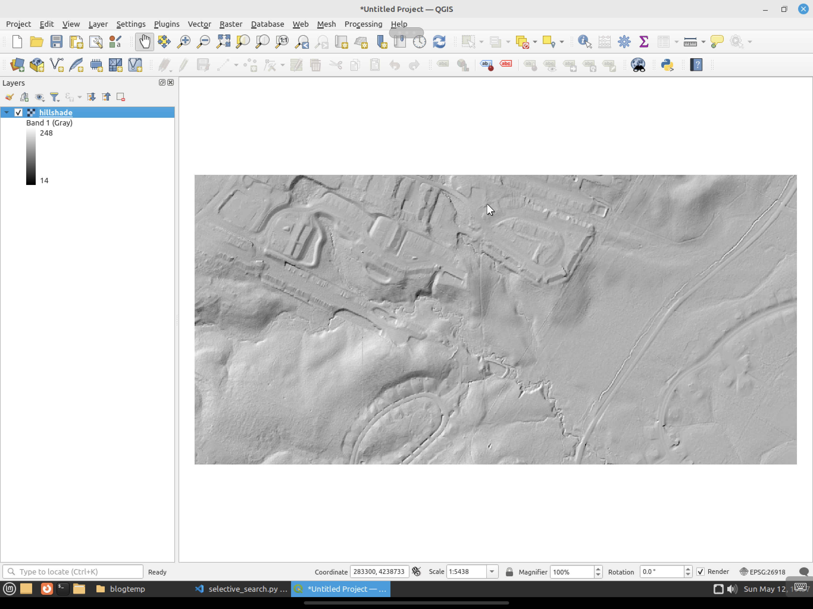
You can see that the hill shade version makes it easier for a human to pick out features versus the original.  It is easier to spot creeks and the flat areas where buildings are.  Now let us see how selective search handles this file.

Selective Search run against a hill shade.

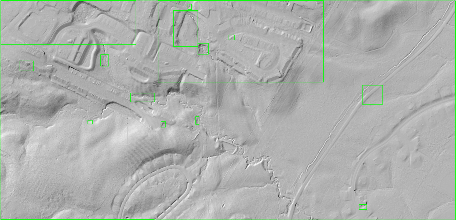
It did somewhat better.  It identified several of the areas where houses are located, but it still missed all of the others.  It also did not pick up on the creeks that run through the area.

Why Did It Not Work So Well?

Now the question you might have is “Why did selective search do so badly in all of the images?”  Well, this type of segmentation is not actually what we would define as object detection today.  It’s more an image processing operation that builds on techniques that have been around for decades that make use of pixel features to identify areas.

Early segmentation methods that led to selective search typically did the following:

  1. Thresholding: Thresholding segments images based on pixel intensity values. This could be a global threshold applied across the entire image or adaptive thresholds that vary over different sized image regions.
  2. Edge Detection: Edge detectors work by identifying boundaries of objects based on discontinuities in pixel intensities, which often correspond to edges.  Some include a pass to try to connect edges to better identify objects.
  3. Region Growing: This method starts with seed points and “grows” regions by appending neighboring pixels that have similar properties, such as color or texture.
  4. Watershed Algorithm: The watershed algorithm treats the image’s intensity values as a topographic surface, where light areas are high and dark areas are low. “Flooding” the surface from the lowest points segments the image into regions separated by watershed lines.

Selective search came about as a hybrid approach that combined computer vision-based segmentation with strategies to group things together.  Some of these were similarity measures such as color, texture, size, and fill to merge regions together iteratively.  It then introduced a hierarchical grouping that built segments at multiple scales to try to better capture objects in an image.

These techniques do still have their uses.  For example, they can quickly find objects on things like conveyor belts in a manufacturing setting, where the object stands out against a uniform background.  However, they tend to fail when an image is “complicated”, like LiDAR as an example or a white goose that does not easily stand out against the background.  And honestly, they are not really made to work with complex images, especially with LiDAR. These use cases require something more complex than traditional segmentation.

This is way longer now than I expected, so I think I will wrap this up here.  Next time I will talk about another computer vision technique to identify areas of an interest in an image, specifically, image saliency.

Applying Deep Learning and Computer Vision to Lidar Part 2: Training Data

In part one I described some of the issues I had on a recent project that applied deep learning to geographic feature recognition in LiDAR and the file sizes of such data.  This time I want to talk about training data, how important it is, and how little there is for this type of problem.

One of the most important things in deep learning is having both quality training data and a good amount of such data.  I have actually written a previous post about the importance of quality data that you can read here.  At a bare minimum, you should typically have around one thousand samples of each object class you want to train a model to recognize.  Object classes in this case are geographic feature types that we want to recognize.

Training Data Characteristics

These samples should mirror the characteristics of the data that your model will come across during classification tasks.  With LiDAR in GeoTIFF format, the training data should be similar in resolution (0.5 meters in this case) and bit depth (32-bit) to the area for testing.  There should be variability in the training data.  Convolutional neural networks are NOT rotational invariant, meaning that unless you train your model on samples at different angles, it will not automatically recognize features.  In this case, your training LiDAR features should be rotated at different angles to account for differences in projection or north direction.

Balanced Numbers of Features per Class

Your training data should also be balanced, meaning that each class should have roughly the same number of training images where possible.  You can perform some tasks that we will talk about in a bit to help with this, but generally if your model is unbalanced, it could mistakenly “lean” towards one class more than others.

Related to this, when generating your training data, you should make sure your training and testing data contain samples from each of your object classes. Especially when imbalanced, it is very easy to use something like train_test_split from the sklearn library and have it generate a training set that misses some object classes. You should also shuffle your training data so that the samples from each class are sufficiently randomized and the model does not assume that features will appear in a specific order. To alleviate this, make sure you pass in something like:

… = train_test_split(…, shuffle=True, stratify=labels)

where labels is a list of your object classes. For most cases this will ensure the order of your samples is sufficiently randomized and that your training/testing data contains samples of each object class.

Complexity

Geographic features also have a varying complexity in how they appear in LiDAR.  The same feature can “look” differently based on its size or other characteristics.  Humans will always look like humans, so training on them is fairly simple.  Geographic features can be in the same class but appear differently based on factors such as weathering, erosion, vegetation, and even if it’s a riverbed that is dry part of the year.  This increased complexity means that samples need to have enough variability, even in the same object class, for proper training.

Lack of Training Data for This Project

With all of this out of the way, let us now talk about the issues that faced this particular project.  First of all, there is not a lot of labeled training data for these types of features.  At all.  I used various search engines, ChatGPT, even bought a bucket of KFC so I could try to throw some bones to lead me to training data (although I don’t know voodoo so probably read them wrong).

There is a lot of data about these geographic features out there, but not labeled AND in LiDAR format.  There is an abundance of photographs of these features.  There are paper maps of these features.  There are research papers with drawings of these features.  I even found some GIS data that had polygons of these features, but the matching elevation model was too low of a resolution to be useful.

In the end I was only able to find a single dataset that matched the bit depth and spatial resolution that matched the test data.  There were a couple of problems with this dataset though.  First, it only had three feature classes out of a dozen or more.  Second, the number of samples of each of these three classes were way imbalanced.  It broke down like this:

  • Class 1 – 123 samples
  • Class 2 – 2,214 samples
  • Class 3 – 9,700 samples

Realistically we should have just tried for Classes 2 and 3, but decided to try to use various techniques to help with the imbalance.  Plus, since it was a bit of a research project, we felt it would be interesting to see what would happen.

Data Augmentation

There are a few different methods of data augmentation you can do to add more training samples, especially with raster data.  Data augmentation is a technique where you generate new samples from existing data so that you can enhance your model’s generalization and generate more data for training. The key part of this is making sure what the methods you use do not change the object class of the training sample.

Geometric Transformations

The first thing you can do with raster data is to apply geometric transformations (again, as long as they do not change the object class of your training sample).  Randomly rotating your training images can help with the rotational invariance mentioned above.  You can also flip your images, change their scale, and even crop them as long as the feature in the training sample remains.

You can gain several benefits from applying geometric transformations to your training data. If your features can appear at different sizes, scaling transforms can help your model become better generalized on feature size. With LiDAR data, suppose someone did not generate the scene with North at the top. Here, random rotations can help the model generalize to rotation so it can better detect features regardless of angle.

Spatial Relationships

Regardless of what type of augmentations you apply to LiDAR, you have to be mindful that you do not change the spatial characteristics of the data. Consider color space augmentation, something that is common with other areas of deep learning and computer vision. With LiDAR, modifying the brightness/contrast would actually be changing the elevation and/or reflectance values of the data. In some applications, especially those highly based on reflectance values such as detecting types of vegetation, this might be useful. In high-resolution geography, you could end up altering the training data in such a way that it no longer represents real-world features.

Wrapping Up

I think I will end this one here as it got longer than I expected and I’m tired of typing 😉  Next time I’ll cover issues with image processing libraries and 32-bit LiDAR data.

Image Processing for Beginners: Image Zooming

Today I’m finally going to finish up the series I started on image processing. The goal of this series is to dispel any myths that algorithms that work on images make things up or do strange, arcane magic. The data is there in the images already, and algorithms that work on them simply make things more visible to a human.

My idea for this originally started when people claimed that zooming in on an image using an iPhone was somehow changing it. The claim (politically motivated) was that it changed the semantic content of the image by zooming in or out. So today I’ll wrap up this series by going over how you zoom an image (or make it larger / smaller).  Note this post will be a bit more technical than the last one as I am including code to demonstrate what I am doing.

Semantic content of an image refers to the meaning or information that the image conveys, such as objects, scenes, actions, attributes, etc. For example, if you take a picture of a cat sitting on a table in your kitchen, then the semantic content would be each of the objects that are in that image (cat, table, kitchen).

Images are resized for you automatically all the time, and you are never aware of it mostly.  Your web browser will scale an image so that it fits on your screen.  Mobile devices scale images such that you can fit them on the device display.  You may even have “pinch to zoom” in on an image so you can see things more clearly.  So ask yourself, when you have zoomed in on an image, do new objects suddenly appear in it?  Does an elephant suddenly appear when you zoom in or out of a picture of your children?  You would have noticed this by now should it happen.

Yes, any time you resize an image you do technically change it, as you have to map pixels from the original to the new size.  However, no resizing operation changes the semantic content of the image.  People have been mapping things and rescaling them long before computers have existed.  Architects, draftsmen, cartographers, and others were transforming and resizing things before electricity was discovered.  Just because a computer does it does not mean that suddenly objects get inserted into the image or that the meaning of the image gets changed.

I’ll be using OpenCV 4 and Python 3. For those unaware, OpenCV is an open source computer vision library that has been around for a long time and is used in thousands of projects. The algorithms in it are some of the best around and have been vetted by experts in the field.  The example image I will be using is a public domain image of a fish as can be seen below.

Public Domain Photo of a Fish

To play along at home, I have the source code for this blog post at https://github.com/briangmaddox/blog_opencv_resizing_example

The first thing we do with our sample image is to load it in using OpenCV, print the dimensions, and then display it.

# Load in our input image
input_image = cv2.imread("1330-sole-fish.jpg")

# Get the dimensions of the original image
height, width, channels = input_image.shape

# Print out the dimensions
print(f"Image Width: {width} Height: {height}")

# Display the original image to the user
cv2.imshow("Original Image", input_image)
cv2.waitKey(0)
cv2.destroyAllWindows()

When we run this code, we see our small fish image in a window:

Image of the fish displayed by OpenCV in a window

Next we will do a “dumb” resize of the image.  Here we double each pixel in the X- and Y-directions.  This has the effect of making the image 2x large, effectively zooming in to the image.

empty_mat = numpy.zeros((height * 2, width * 2, channels), dtype=numpy.uint8)

Here empty_mat is an empty image that has been initialized to all zeroes.  Numpy is a well known array library that OpenCV and other packages are built on.  When OpenCV and Python load an image, they store it in what is basically a three dimensional array.  You can think of this as a box where each red, green, and blue channel of the image is contained in the box.

We do the following loop now to copy the pixel to the output empty_mat:

for y in range(height):
    for x in range(width):
        pixel = input_image[y, x]
        empty_mat[y * 2, x * 2] = pixel
        empty_mat[y * 2, x * 2 + 1] = pixel
        empty_mat[y * 2 + 1, x * 2] = pixel
        empty_mat[y * 2 + 1, x * 2 + 1] = pixel

I used a simple loop and assignments to make it easier to see what I am doing.  This loop simply goes through each row of the input image and copies that pixel to four pixels in the output image, effectively doubling the size and zooming the image.

Now we display both the original image and the doubled one.

cv2.imshow("Original Image", input_image)
cv2.imshow("Doubled image", empty_mat)
cv2.waitKey(0)

cv2.destroyAllWindows()
Both the original image and the doubled image displayed by OpenCV

In the above screenshot, we can see that the image has indeed been “zoomed” in and is now twice the size of the original.  Semantically, both images are equal to each other.  You can see the jaggedness of the fish in the doubled image due to the simplistic nature of the resize.  The main take away from this is that it is still the same image, even if it is larger than the original.

Most applications that let you zoom in or resize images use something a bit smarter than a simple doubling of each pixel.  As you can see with the above images, the simple “doubling” results in a jagged image that becomes less visually pleasing as the zoom multiplier gets larger.  This is because to double an image using the simple method, each pixel becomes four pixels.  Four times larger means eight pixels, and so on.  This method also becomes much more complicated if the zoom factor is not an even multiple of two.

Images today are resized using mathematical interpolations.  Wikipedia defines interpolation as “a type of estimation, a method of constructing (finding) new data new points based on the range of a discrete set of known data points.”  “Ah ha!” you might say, this sounds like things are being made up.  And yes they are, but data is not being made up out of the blue.  Instead, interpolations use existing data to mathematically predict data to fill in the gaps. Google, Apple, and other mapping applications use interpolations to fill in the gaps of your position to display on the screen in-between calculating your exact position using the satellites.  Our brains do it when we reach out to catch a fast ball.  Weather and financial forecasters use it every day.

Interpolations have a long history in mathematics.  The Babylonians were using linear and other interpolations as far back as the 300’s BCE to predict the motions of celestial bodies.  As time has gone on, mathematicians have devised better and more accurate methods of predicting values based on existing ones.  Over time, we have gone from the relatively simplistic piecewise constant interpolations to Gaussian processes.  Each advance has made better and closer predictions to what the missing values actually are.

Consider an example using linear interpolation.  This type of problem is often taught in geometry and other math classes.  Assume that we have points on a two-dimensional XY axis such as below.

Plot of the function y=x with the points (2,2) missing.

Here we see we are given a series of (1,1), (3,3), (4,4), (5,5), (6,6), and (7,7).  This is in fact a plot of the function y = x, except I omitted the point (2,2).  We can eyeball and see that the missing y value for x=2 is in fact 2, but let us go through the math.

The formula for linear interpolation is: .  So if we want to solve for the point where x=2, (x1,y1) will be the point (1,1) and (x2, y2) will be the point (3,3).  Plugging these numbers in we get , which indeed gives us y=2 for x=2.  No magic here, just math.

Other types of interpolations, such as cubic, spline, and so on, also have mathematical equations that calculate new values based on existing values.  This point is important to note.  All interpolations use math to calculate new values based on existing ones.  These interpolations have been used over hundreds of years, and are the basis for many things we use today.  No magic, no guessing, no making things up.  I think we can trust them.

So let us get back to image processing.  OpenCV fortunately can use interpolation to resize an image.  As a reminder, we typically do this so that the image is more pleasing to the eye.  Interpolations give us images that are not blocky as in the case of the simple image doubling technique.  First we will use linear interpolation to double the size of the image

double_width = width * 2
double_height = height * 2
linear_double_image = cv2.resize(input_image, (double_width, double_height), interpolation=cv2.INTER_LINEAR)

# Now display both the original and the linear interpolated image to compare.
cv2.imshow("Original Image", input_image)
cv2.imshow("Linear Interpolated image", linear_double_image)
cv2.waitKey(0)
cv2.destroyAllWindows()

To make things explicit, we set new dimensions to twice the width and height of the image and use linear interpolation to scale the image up.

Original image and a linearly interpolated 2x image displayed with OpenCV

Here we see that the interpolated image is not as blocky as the simple pixel doubling image, meaning that yes the new image is a bit different from the original.  However, nothing new has been added to the image.  It has not been distorted and the same semantic content has been preserved.  We can look at what has happened by examining the coordinates at pixel (0,0) in the original image.

Let us take this farther now.  What happens if we increase to four times the original size?

# Linear interpolation to quad size
quad_width = width * 4
quad_height = height * 4

linear_quad_image = cv2.resize(input_image, (quad_width, quad_height), interpolation=cv2.INTER_LINEAR)

# Now display both the original and the linear interpolated image to compare.
cv2.imshow("Original Image", input_image)
cv2.imshow("Linear Interpolated 4x image", linear_quad_image)
cv2.waitKey(0)
cv2.destroyAllWindows()
Original image and a linearly interpolated 4x image displayed by OpenCV

Again, creating a 4x-size image does not introduce any new objects or change the semantic meaning of the image. You may notice that it looks a bit more blurry than the 2x image.  This is because linear interpolation is a simple process. 

Let us see what it looks like using a more rigorous cubic interpolation to create a 4x image.

# Cubic interpolation
cubic_quad_image = cv2.resize(input_image, (quad_width, quad_height), interpolation=cv2.INTER_CUBIC)

# Now display both the original and the linear interpolated image to compare.
cv2.imshow("Original Image", input_image)
cv2.imshow("Cubic Interpolated 4x image", cubic_quad_image)
cv2.waitKey(0)
cv2.destroyAllWindows()
Original image and the cubic interpolated 4x image displayed by OpenCV

We can see that the image does not have as pronounced blockiness that the linearly interpolated image has.  Yes, it is not exactly the same as the original image as we did not simply double each pixel.  However, the semantic contents of the image are the same, even using a different interpolation method.  We did not introduce anything new into the image by resizing it.  The meaning of the image is the same as it was before.  It is just larger so we can see it better.

It is time to wrap this up as it is a longer post than I intended.  You can see from the above that resizing (or zooming in on) an image does not change the content of the image.  We did not turn the fish into a shark by enlarging it.  We did not add another fish to the image by enlarging it.  

I encourage you to try this on your own at home.  Pull out your phone, take a picture, and then zoom in on it.  Your camera likely takes such a high resolution that displaying it on your screen actually reduces some detail, so that you have to zoom in to see the fine detail in the image.  Ask yourself though, is the meaning of the image changed by zooming in or out on it?  Are they still your children, or did zooming in turn them into something else?

I hope that the next time you hear something in the news about image processing, you realize that every algorithm that does this is just math. It is either math to bring out fine details that you cannot normally see in the case of dark images, or math that makes the image larger so that you can better see the smile on a child.  The content of the image is not changed, it is always semantically the same as the original image.

Some Thoughts on Creating Machine Learning Data Sets

My whole professional career (26 years now!) has been in slinging data around. Be it writing production systems for the government or making deep learning pipelines, I have made a living out of manipulating data. I have always taken pains to make sure what I do is correct and am proud of how obsessive I am about putting things together.

Lately I have been back to doing deep learning and computer vision work and have been looking at some of the open datasets that are out there for satellite imagery. Part of this work has involved trying to combine datasets to train models for object classification from various satellite imagery providers.

One thing I have noticed is that it is still hard to make a good deep learning dataset. We are only human, and we miss things sometimes. It is easy to misclassify things or accidentally include images that might not be a good candidate. Even ImageNet, one of the biggest computer vision and deep learning datasets out there, has been found to contain errors in the training data.

This got me thinking about putting together datasets and what “rules of thumb” I would use for doing so. As there do not seem to be as many articles out there about making datasets versus using them, I thought I would add my two cents on making a good machine learning dataset. This is by no means a criticism about the freely-available datasets out there now. In fact, we should all be thankful so many people are putting them out there, and I hope to add to these soon! So, in no particular order, here we go.

Limit the Number of Object Classes

One thing I have noticed is many datasets try to break out their object classes into too fine of detail. This looks to be especially true for satellite datasets. For example, one popular dataset breaks aircraft down into multiple classes ranging from propeller to trainer to jet aircraft. One problem with this approach is that it becomes easy to pick the wrong category while classifying them. Jet trainers are out there. Should that go into the jet category, or the trainer category? There are commercial propeller aircraft out there. What do we do with them?

It is one thing if you are purposely trying to differentiate different types of aircraft from satellite imagery. Even then, however, I would guess that a neural network would learn mostly the same features for each object class, and you would end up getting the aircraft category correct but have numerous misclassifications for the type. It will also be a lot easier to accidentally mislabel things from imagery while you are building the dataset. Now this is different if you are working with imagery to which only certain types of three letter agencies have access. But, most of us have to make due with the types of imagery that are freely available.

Verify Every Dataset Before Use

We all get into a hurry. We have deadlines, our projects are usually underfunded, and we spend large amounts of time putting out fires. It is still vitally important to not blindly use a dataset to train your model! Consider the below image. In one public domain dataset out there, around eight of these images are all labeled as boats.

Image of a car labeled as a boat.

This is a classical example of “we’re only human.” I would wager that a lot of datasets contain errors such as this. It is not that anyone is trying to purposely mislead you. It just happens sometimes. This is why it is essential to go through your dataset no matter how boring it might be. Labeling is a tough job, and there is probably a room in Hell that tortures people by making them label things all day and night. Again, everyone makes mistakes.

Clean up Your Datasets

Some datasets out there are derived from Google Earth. It is a source of high quality imagery and for now the terms seem to not require your firstborn or an oath of loyalty. The problem comes when you include things like the image below in your training set.

Here you can see that someone used an aircraft that had the Google Earth watermark superimposed on top of it. If you only have one or two, it likely will not be an issue. However, if you have a lot of things like this, then your network could learn features from the text and start to expect imagery to have this in it. This is an example of where you should practice due diligence in cleaning up your data before putting it into a machine learning dataset.

Avoid Clusters (Unless Looking for Them)

When extracting objects from Google Earth, you might come across something you consider a gold mine. Say you are extracting and labeling cars from imagery, and you come across a full parking lot. This seems like an easy way to suddenly add a lot of training data, and you might end up with a lot of images such as the one below.

In a dataset I recently worked with, there were several object classes that had a lot of images of the same types of objects right next to each other. If you do this, keep in mind that there could be some side effects from having a lot of clusters in your dataset.

  • It could (possibly) be helpful because your object class can present different views if they are present in a cluster. In the above, you can see the top of one bus and the back of another right beside it. This can aid in learning different features for that class.
  • A negative is that if you have a lot of clusters of objects in your training data, your classifier might lean towards detecting objects in groups instead of individual objects. If you are specifically looking for clusters then this is OK. If you want to search for individual ones, then it could hurt your accuracy.
  • The complexity of your training data could increase and lead to slow-downs during the training process by having more features present for each example object than would be present ordinarily.

In general, it is OK to have some clusters of objects in your data. Just be mindful that if you are looking for individual objects, you should try not to have a lot of clusters in your training data.

Avoid Duplicate Objects

This is true for objects in the same class or between object classes. If you have a lot of duplicates, you can run the risk of over-fitting during training. Problems can also arise if you, say, have a car in both a car object class and in a truck class. In this case you can end up with false detections because you accidentally matched the same features in multiple classes.

Pick Representative Training Data

If you are trying to train a model to detect objects from overhead imagery, you would not want to use a training set of pictures people have taken from their cellular phones. Similarly, if you want to predict someone’s mood from a high resolution camera, you would not want to train using fuzzy webcam images. This is stressed in numerous deep learning texts out there, but it is important to repeat. Check if the data you are using for training matches the data you intend to be running your model on. Fitness for use is important.

Invariance

The last thing I want to discuss here is what I feel is one of the most important aspects of deep learning: invariance. Convolutional neural networks are NOT invariant to scale and rotation. They can detect translations, but you do not get scale or rotational invariance by default. You have to provide this using data augmentation during your training phase.

Consider a dataset of numbers that you are using to train a model. This dataset will likely have the numbers written as you would expect them to be: straight up and down. If you train a model on this, it will detect numbers that match a vertical orientation, but accuracy will go down for anything that is off the vertical axis.

Frameworks like Keras make this easy by providing classes or functions that can randomly rotate, shear, or scale images during training before they are input into the network. This helps the classifier learn features in different orientations, something that is important for classifying overhead imagery.

Conclusion

In summary, these are just some general guidelines I use when I am putting together a dataset. I do not always get everything right, and neither will you. Get multiple eyes looking at your dataset and take your time. Labeling is a laborious, and if your attention drifts it is easy to get wrong. The better quality your training data, the better your model will perform.

Building OpenCV 2.3.1 on Ubuntu 11.04

Getting OpenCV 2.3.1 to compile on Ubuntu can be interesting.  The first issue is tracking down all of the dependencies you need to get the different parts of it to work properly.  There is more information on dependencies needed at the OpenCV wiki here and here.  I found this page on a blog as well which will help to get a lot of the dependencies down.

For me specifically, I had a couple of problems on 11.04.  Make sure you have the following packages installed to enable gstreamer and unicap support:

libgstreamer-plugins-base0.10-dev
libgstreamer0.10-dev
libunicap2
libunicap2-dev
libucil2-dev

The second major problem is that OpenCV 2.3.1 doesn’t fully track the latest releases of ffmpeg.  This patch helps, but bear in mind that it’s for OpenCV 2.3.0 and there have been changes between versions.  You’ll have to install the patch by hand to take care of some of the differences.

Once this is done, you should be ready to build.  On my system I ran cmake as:

cmake -D CMAKE_BUILD_TYPE=RELEASE -D CMAKE_INSTALL_PREFIX=/usr/local -D BUILD_PYTHON_SUPPORT=ON -D WITH_TBB=ON -D WITH_XINE=ON -D WITH_UNICAP=ON -D BUILD_EXAMPLES=ON -D BUILD_NEW_PYTHON_SUPPORT=ON -D INSTALL_PYTHON_EXAMPLES=ON -D BUILD_DOCUMENTATION=ON -D BUILD_SHARED_LIBS=ON ..

If you have all of the extra media repositories on Ubuntu enabled, I’d highly recommend NOT disabling shared libraries when building OpenCV.  You’ll avoid some linking errors due to concurrent versions of some of the multimedia libraries that might be installed.

After that, when you compile make sure you add in something like -I/usr/local/include and -L/usr/local/lib to your makefile to make sure you’re pulling in the version you just compiled instead of the default and you should be good to go.