The USGS Board on Geographic Names maintains the Geographic Names Information System (GNIS) database.  It is a database of over two million points in the United States.  This database:

contains information about physical and cultural geographic features in the United States and associated areas, both current and historical (not including roads and highways). The database holds the Federally recognized name of each feature and defines the location of the feature by state, county, USGS topographic map, and geographic coordinates.

You can download the 79 megabyte GNIS zip file from here.  You will want to select the NationalFile as it is not broken up into individual states.  Importing GNIS into PostGIS is slightly more complicated as it does not come as a Shapefile, but instead as a 293 megabyte text file once it is unzipped from the  above.  Download the file, unzip it, and open a command window where the unzipped file is.  Note that the last time I did this on Windows, using the command line client was an exercise in pain due to how Windows handles code pages and character types.  On Windows it might be easier to do this inside something like pgadmin.

To import, first create a database inside PostgreSQL using something like the following:

createdb -T gistemplate USGS

Once done, you will want to run

psql -d USGS

to start the PostgreSQL database client.  Now you will want to create the table to hold the data.  To do this, copy and paste this statement into the psql client window:

CREATE TABLE gnis
(
 feature_id integer NOT NULL,
 feature_name character varying,
 feature_class character varying,
 state_alpha character(2),
 state_numeric character(2),
 county_name character varying,
 county_numeric character(3),
 primary_lat_dms character varying,
 prim_long_dms character varying,
 prim_lat_dec real,
 prim_long_dec real,
 source_lat_dms character varying,
 source_long_dms character varying,
 source_lat_dec real,
 source_long_dec real,
 elev_in_m integer,
 elev_in_ft integer,
 map_name character varying,
 date_created date,
 date_edited date
);

Note that I COULD have spent the time figuring out the maximum size of each column, instead of just making them varchars, to save space.  But, again, I’m lazy 🙂

Now to import, you will run the following command.  The .txt files is over two million rows, so it could take a while to import depending on the speed of your system.

 USGS=# \copy gnis from NationalFile_20140204.txt DELIMITER '|' CSV HEADER

If you get a file not found error,run \copy with the full path to the NationalFile.  Depending on when you do this, the file name may be different based on when it was last updated.

We are not done yet.  There is no actual geospatial geometry column in the database.  We will need to create one from the existing columns.  To do this, first we must create a geometry column to hold the geospatial points.

USGS=# SELECT AddGeometryColumn('public', 'gnis', 'geom', 4326, 'POINT', 2);

This command tells PostgreSQL to add a geometry column named geom to the gnis table in the public schema using NAD83.  Now we need to actually populate this column.  We need to take the latitude and longitude columns in the table and convert them into a binary representation that PostGIS uses internally.

USGS=# update public.gnis 
SET geom = ST_PointFromText('POINT(' || prim_long_dec || ' ' || prim_lat_dec || ')', 4326);

Here we have PostgreSQL convert the prim_long_dec and prim_lat_dec columns into a POINT and then to the actual geometry using the ST_PointFromText function inside PostGIS.

Now we need to add a geospatial index on the geom column.  You need an index to use the data in apps such as QGIS as it makes area look-ups much faster.

USGS=# create index gnis_geom_gist_idx on gnis using gist(geom);

Now that we have an index, we need to create our database statistics and cluster it on the geom column.  As I mentioned in a previous post, you will run these commands in order (waiting for each one to complete before running the next):

USGS=# vacuum analyze gnis;
USGS=# cluster gnis using gnis_geom_gist_idx;
USGS=# analyze gnis;

And now we are done.  You have your own local copy of GNIS that you can use in visual GIS tools or from the command line.  There are some fun things you can do with the data, such as the below figure shows where I used QGIS to load all points in GNIS that have my last name in them (my modesty astounds even me 😉

Maddox Places in QGIS

Happy GISing!

Check out my GIS data section here.  I’ve uploaded state-based Shapefiles of the Census ROADS, LINEARWATER, and others.

Now that you have a lot of data into your geospatial database, we should take a little bit of time to discuss how to manage it and keep it running smoothly.  This can make the difference between requests timing out and having data be returned almost instantaneously.

Database Tuning

There are a large number of sources online that will go over how to configure PostgreSQL for maximum performance.  The PostgreSQL team themselves provide such documentation at the Tuning Your PostgreSQL Server wiki page and a list of many techniques at their Performance Optimization wiki page.

For the PostGIS side of things, Boundless has a workshop page titled Tuning Postgres for Spatial that provides some information on configuring for spatial operations.  The PostGIS team also has some tips that can be found at this link.

Another tool is the pgtune utility.  This is a command line tool that lets you specify what you will be using your database for and what type of machine it is running on.  It then will give you several options that you can put in the PostgreSQL configuration files.

Table Maintenance

In general, the main things you should consider are creating indices, vacuuming your database to remove unused space, keeping your database statistics up to date, and clustering your database so that data that is spatially near each other are physically near each other on disk.

To perform the following commands, open a command prompt and run the command:

psql -d Census_2013

You should then see output similar to the following:

[bmaddox@girls ~]$ psql -d Census_2013 
psql (9.2.7)
Type "help" for help.

Census_2013=#

If you followed the commands in this series, your database tables should already have a spatial index based on the geom column that lets PostGIS only return data that you have requested.  To see this, first run the command

\dt

This will give you a list of all of the tables in your database.  On my system, I get the output below:

Census_2013=# \dt
 List of relations
 Schema | Name | Type | Owner 
--------+-----------------------------------------+-------+---------
 public | county_outlines | table | bmaddox
 public | spatial_ref_sys | table | bmaddox
 public | state_outlines | table | bmaddox
 public | us_113_congress_districts | table | bmaddox
 public | us_alaska_native_regional_corporations | table | bmaddox
 public | us_area_landmarks | table | bmaddox
 public | us_area_water | table | bmaddox
 public | us_census_block_groups | table | bmaddox
 public | us_coastlines | table | bmaddox
 public | us_combined_new_england_city_town_areas | table | bmaddox
 public | us_combined_statistical_areas | table | bmaddox
 public | us_elementary_school_districts | table | bmaddox
 public | us_indian_alaska_hawaii_native_areas | table | bmaddox
 public | us_indian_tribal_subdivisions | table | bmaddox
 public | us_linear_water | table | bmaddox
 public | us_metro_micropolitan_statistical_areas | table | bmaddox
 public | us_military_areas | table | bmaddox
 public | us_new_england_city_town_areas | table | bmaddox
 public | us_new_england_city_town_divisions | table | bmaddox
 public | us_primary_roads | table | bmaddox
 public | us_primary_secondary_roads | table | bmaddox
 public | us_rails | table | bmaddox
 public | us_roads | table | bmaddox
 public | us_secondard_school_districts | table | bmaddox
 public | us_state_legislative_lower | table | bmaddox
 public | us_state_legislative_upper | table | bmaddox
 public | us_tribal_block_groups | table | bmaddox
 public | us_unified_school_districts | table | bmaddox
 public | us_urban_areas_2010 | table | bmaddox
 public | us_zip_code_areas | table | bmaddox
(30 rows)

Census_2013=#

To get further details on a table, including the indices, run the following:

Census_2013=# \d us_zip_code_areas
 Table "public.us_zip_code_areas"
 Column | Type | Modifiers 

------------+-----------------------------+---------------------------------------------------------
--------
 gid | integer | not null default nextval('us_zip_code_areas_gid_seq'::re
gclass)
 zcta5ce10 | character varying(5) | 
 geoid10 | character varying(5) | 
 classfp10 | character varying(2) | 
 mtfcc10 | character varying(5) | 
 funcstat10 | character varying(1) | 
 aland10 | double precision | 
 awater10 | double precision | 
 intptlat10 | character varying(11) | 
 intptlon10 | character varying(12) | 
 geom | geometry(MultiPolygon,4269) | 
Indexes:
 "us_zip_code_areas_pkey" PRIMARY KEY, btree (gid)
 "us_zip_code_areas_geom_gist" gist (geom)

Census_2013=#

The geospatial index here is the us_zip_code_areas_geom_gist  while the standard primary key index is us_zip_code_areas_pkey.

When you create a new index, or perform a large number of inserts, updates, or deletes, you generally need to update the database’s statistics on that table as well as clear out any unused space.  Pick one of your tables and run the following command, noting that depending on the size of your database (especially with US_Roads, for example), this command can take a while to complete:

Census_2013=# vacuum analyze us_zip_code_areas;
VACUUM
Census_2013=#

This command tells PostgreSQL to clean up any unused space and update statistics on the us_zip_code_areas table.  These statistics are used internally by the database when it runs user queries on the data.

The next thing you should do is cluster the data.  Clustering is an operation that is performed against a database index and it physically places data that is close to each other in the index in the same area on the hard drive.  For geospatial data, this can make a huge difference, as the database does not have to scan multiple areas on the hard drive to return data that your GIS may request.  To cluster data on the geospatial index, run the following command next, again noting that this could take a while to finish depending on the size of your database and your hardware:

Census_2013=# cluster us_zip_code_areas using us_zip_code_areas_geom_gist ;
CLUSTER
Census_2013=#

Once finished, run the table describe command (\d) again:

Census_2013=# \d us_zip_code_areas
 Table "public.us_zip_code_areas"
 Column | Type | Modifiers 

------------+-----------------------------+---------------------------------------------------------
--------
 gid | integer | not null default nextval('us_zip_code_areas_gid_seq'::re
gclass)
 zcta5ce10 | character varying(5) | 
 geoid10 | character varying(5) | 
 classfp10 | character varying(2) | 
 mtfcc10 | character varying(5) | 
 funcstat10 | character varying(1) | 
 aland10 | double precision | 
 awater10 | double precision | 
 intptlat10 | character varying(11) | 
 intptlon10 | character varying(12) | 
 geom | geometry(MultiPolygon,4269) | 
Indexes:
 "us_zip_code_areas_pkey" PRIMARY KEY, btree (gid)
 "us_zip_code_areas_geom_gist" gist (geom) CLUSTER

Census_2013=#

As you can see, the geom index now has the world CLUSTER behind it, denoting that this is the index that you clustered on.  It will generally make more sense for geospatial databases to cluster on the geospatial index as that will ensure data that is near each other in the real world is near each other on disk.

However, now that you have moved data around on disk, you again need to update the database statistics.  You will not need to vacuum it again, as the cluster command does this itself as it rearranges the data.

Census_2013=# analyze us_zip_code_areas ;
ANALYZE
Census_2013=#

So there you are.  Running these commands on your data tables, in addition to tuning your database itself, can make a huge performance difference over simply accepting the default options.

Next time we will go over backing up your database and then head on to loading data again, such as the USGS Geographic Names Information System (GNIS), the National Geospatial-Intelligence Agency’s Geonames, and OpenStreetMap.

Now we move on to the rest of the Census data that I’m discussing for this series: ROADS, LINEARWATER, AREAWATER, and AREALM.  If you have not already, go ahead and use lftp to mirror these directories.  Keep in mind that ROADS and LINEARWATER are several gigabytes in size so make sure you have enough room to stage them.

We will start with the ROADS data.  By now you know how to download the data and stage it so we will skip that part.  When you are done you will find all of the following files:

[bmaddox@girls ROADS]$ ls
tl_2013_01001_roads.zip tl_2013_19039_roads.zip tl_2013_30037_roads.zip tl_2013_46127_roads.zip
tl_2013_01003_roads.zip tl_2013_19041_roads.zip tl_2013_30039_roads.zip tl_2013_46129_roads.zip
tl_2013_01005_roads.zip tl_2013_19043_roads.zip tl_2013_30041_roads.zip tl_2013_46135_roads.zip
tl_2013_01007_roads.zip tl_2013_19045_roads.zip tl_2013_30043_roads.zip tl_2013_46137_roads.zip
tl_2013_01009_roads.zip tl_2013_19047_roads.zip tl_2013_30045_roads.zip tl_2013_47001_roads.zip
...
tl_2013_19031_roads.zip tl_2013_30029_roads.zip tl_2013_46119_roads.zip tl_2013_72153_roads.zip
tl_2013_19033_roads.zip tl_2013_30031_roads.zip tl_2013_46121_roads.zip tl_2013_78010_roads.zip
tl_2013_19035_roads.zip tl_2013_30033_roads.zip tl_2013_46123_roads.zip tl_2013_78020_roads.zip
tl_2013_19037_roads.zip tl_2013_30035_roads.zip tl_2013_46125_roads.zip tl_2013_78030_roads.zip
[bmaddox@girls ROADS]$ 
3232 files

First thing to do now is make sure all of the files are not corrupt.  Sometimes downloads can be silently corrupted (although I have found lftp seems to be more reliable than things I have used in the past).  The following command will help identify any issues with the files:

[bmaddox@girls ROADS]$ for foo in *.zip; do unzip -tq $foo; done |grep -v "No errors"
[bmaddox@girls ROADS]$

If you get output like the above, your zip files are at least correct.  The next thing now is to run the following script, called makestates.sh, to create directories for all of the US states and territories and move the files into them.  It is simple, but it works 🙂

makestates.sh

#!/bin/sh
echo "Making state directories."
mkdir 01_Alabama
mkdir 02_Alaska
mkdir 04_Arizona
mkdir 05_Arkansas
mkdir 06_California
mkdir 08_Colorado
mkdir 09_Connecticut
mkdir 10_Delaware
mkdir 11_District_of_Columbia
mkdir 12_Florida
mkdir 13_Georgia
mkdir 15_Hawaii
mkdir 16_Idaho
mkdir 17_Illinois
mkdir 18_Indiana
mkdir 19_Iowa
mkdir 20_Kansas
mkdir 21_Kentucky
mkdir 22_Louisiana
mkdir 23_Maine
mkdir 24_Maryland
mkdir 25_Massachusetts
mkdir 26_Michigan
mkdir 27_Minnesota
mkdir 28_Mississippi
mkdir 29_Missouri
mkdir 30_Montana
mkdir 31_Nebraska
mkdir 32_Nevada
mkdir 33_New_Hampshire
mkdir 34_New_Jersey
mkdir 35_New_Mexico
mkdir 36_New_York
mkdir 37_North_Carolina
mkdir 38_North_Dakota
mkdir 39_Ohio
mkdir 40_Oklahoma
mkdir 41_Oregon
mkdir 42_Pennsylvania
mkdir 44_Rhode_Island
mkdir 45_South_Carolina
mkdir 46_South_Dakota
mkdir 47_Tennessee
mkdir 48_Texas
mkdir 49_Utah
mkdir 50_Vermont
mkdir 51_Virginia
mkdir 53_Washington
mkdir 54_West_Virginia
mkdir 55_Wisconsin
mkdir 56_Wyoming
mkdir 60_American_Samoa
mkdir 64_Federated_States_of_Micronesia
mkdir 66_Guam
mkdir 68_Marshall_Islands
mkdir 69_Commonwealth_of_the_Northern_Mariana_Islands
mkdir 70_Palau
mkdir 72_Puerto_Rico
mkdir 74_US_Minor_Outlying_Islands
mkdir 78_US_Virgin_Islands
echo "Moving files to state directories"
mv tl_2013_01* 01_Alabama
mv tl_2013_02* 02_Alaska
mv tl_2013_04* 04_Arizona
mv tl_2013_05* 05_Arkansas
mv tl_2013_06* 06_California
mv tl_2013_08* 08_Colorado
mv tl_2013_09* 09_Connecticut
mv tl_2013_10* 10_Delaware
mv tl_2013_11* 11_District_of_Columbia
mv tl_2013_12* 12_Florida
mv tl_2013_13* 13_Georgia
mv tl_2013_15* 15_Hawaii
mv tl_2013_16* 16_Idaho
mv tl_2013_17* 17_Illinois
mv tl_2013_18* 18_Indiana
mv tl_2013_19* 19_Iowa
mv tl_2013_20* 20_Kansas
mv tl_2013_21* 21_Kentucky
mv tl_2013_22* 22_Louisiana
mv tl_2013_23* 23_Maine
mv tl_2013_24* 24_Maryland
mv tl_2013_25* 25_Massachusetts
mv tl_2013_26* 26_Michigan
mv tl_2013_27* 27_Minnesota
mv tl_2013_28* 28_Mississippi
mv tl_2013_29* 29_Missouri
mv tl_2013_30* 30_Montana
mv tl_2013_31* 31_Nebraska
mv tl_2013_32* 32_Nevada
mv tl_2013_33* 33_New_Hampshire
mv tl_2013_34* 34_New_Jersey
mv tl_2013_35* 35_New_Mexico
mv tl_2013_36* 36_New_York
mv tl_2013_37* 37_North_Carolina
mv tl_2013_38* 38_North_Dakota
mv tl_2013_39* 39_Ohio
mv tl_2013_40* 40_Oklahoma
mv tl_2013_41* 41_Oregon
mv tl_2013_42* 42_Pennsylvania
mv tl_2013_44* 44_Rhode_Island
mv tl_2013_45* 45_South_Carolina
mv tl_2013_46* 46_South_Dakota
mv tl_2013_47* 47_Tennessee
mv tl_2013_48* 48_Texas
mv tl_2013_49* 49_Utah
mv tl_2013_50* 50_Vermont
mv tl_2013_51* 51_Virginia
mv tl_2013_53* 53_Washington
mv tl_2013_54* 54_West_Virginia
mv tl_2013_55* 55_Wisconsin
mv tl_2013_56* 56_Wyoming
mv tl_2013_60* 60_American_Samoa
mv tl_2013_64* 64_Federated_States_of_Micronesia
mv tl_2013_66* 66_Guam
mv tl_2013_68* 68_Marshall_Islands
mv tl_2013_69* 69_Commonwealth_of_the_Northern_Mariana_Islands
mv tl_2013_70* 70_Palau
mv tl_2013_72* 72_Puerto_Rico
mv tl_2013_74* 74_US_Minor_Outlying_Islands
mv tl_2013_78* 78_US_Virgin_Islands

Running it will give the following output:

[bmaddox@girls ROADS]$ ~/bin/makestates.sh 
Making state directories.
Moving files to state directories
mv: cannot stat ‘tl_2013_64*’: No such file or directory
mv: cannot stat ‘tl_2013_68*’: No such file or directory
mv: cannot stat ‘tl_2013_70*’: No such file or directory
mv: cannot stat ‘tl_2013_74*’: No such file or directory
[bmaddox@girls ROADS]$

For example purposes, change to the 01_Alabama directory now.  We will go through how to convert one state to a single Shapefile and then leave the rest for you to do on your own 🙂  First we will use the doogr.sh script that I mentioned last week.  Here it is again:

doogr.sh

#!/bin/bash

# Script to automatically create state-based shapefiles using ogr2ogr
# Grab the name of the output shapefile
shapefilename=$1

# Now grab the name of the initial input file
firstfile=$2

# make the initial state file
echo "Creating initial state shapefile $shapefilename"
ogr2ogr $shapefilename $firstfile

# Grab the basename of the firstfiles
firstfilebase=`basename $firstfile .shp`

# Grab the basename of the shapefile for ogr2ogr update
shapefilenamebase=`basename $shapefilename .shp`

# Delete the first files
echo "Now deleting the initial shapefiles to avoid duplication"
rm $firstfilebase.*
#ls $firstfilebase.*

# Now make the rest of the state shape files
echo "Merging the rest of the files into the main shapefile"
for foo in tl*.shp; do
 ogr2ogr -update -append $shapefilename $foo -nln $shapefilenamebase
done

The following commands show how to convert all of the county-level Shapefiles in the 01_Alabama into a single state-level Shapefile.

[bmaddox@girls 01_Alabama]$ doogr.sh 01_Alabama_Roads.shp tl_2013_01001_roads.shp
Creating initial state shapefile 01_Alabama_Roads.shp
Now deleting the initial shapefiles to avoid duplication
Merging the rest of the files into the main shapefile
[bmaddox@girls 01_Alabama]$ \rm tl*
[bmaddox@girls 01_Alabama]$ ls -l
total 186472
-rw-rw-r-- 1 bmaddox bmaddox 53279870 Mar 3 10:34 01_Alabama_Roads.dbf
-rw-rw-r-- 1 bmaddox bmaddox 165 Mar 3 10:34 01_Alabama_Roads.prj
-rw-rw-r-- 1 bmaddox bmaddox 134344780 Mar 3 10:34 01_Alabama_Roads.shp
-rw-rw-r-- 1 bmaddox bmaddox 3304268 Mar 3 10:34 01_Alabama_Roads.shx
[bmaddox@girls 01_Alabama]$ shp2pgsql -s 4269 -c -D -I -WLATIN1 01_Alabama_Roads.shp US_Roads |psql -d Census_2013
Shapefile type: Arc
Postgis type: MULTILINESTRING[2]
SET
SET
BEGIN
NOTICE: CREATE TABLE will create implicit sequence "us_roads_gid_seq" for serial column "us_roads.gid"
CREATE TABLE
NOTICE: ALTER TABLE / ADD PRIMARY KEY will create implicit index "us_roads_pkey" for table "us_roads"
ALTER TABLE
addgeometrycolumn
-------------------------------------------------------------
public.us_roads.geom SRID:4269 TYPE:MULTILINESTRING DIMS:2
(1 row)

CREATE INDEX
COMMIT
[bmaddox@girls 01_Alabama]$

Now it is your turn to do the rest of the directories.  Note, however, that for the others, you will have to slightly change your shp2pgsql command to append instead of insert, as the example below shows:

shp2pgsql -s 4269 -a -D -WLATIN1 02_Alaska_Roads.shp US_Roads |psql -d Census_2013

You will need to use the -a command to APPEND instead of INSERT and CREATE into the database.  Now move on and do the LINEARWATER and AREAWATER data the same way.  The first state you load use the -c -D -I options, the rest the -a -D ones.  As a reminder, as I write these posts, I am uploading the files to my website at https://brian.digitalmaddox.com/blog/?page_id=202.

Now move on to the AREALM directory to process the area landmark files.  Mirrored, the directory will have the following files:

bmaddox@girls AREALM]$ ls
tl_2013_01_arealm.zip tl_2013_18_arealm.zip tl_2013_32_arealm.zip tl_2013_47_arealm.zip
tl_2013_02_arealm.zip tl_2013_19_arealm.zip tl_2013_33_arealm.zip tl_2013_48_arealm.zip
tl_2013_04_arealm.zip tl_2013_20_arealm.zip tl_2013_34_arealm.zip tl_2013_49_arealm.zip
tl_2013_05_arealm.zip tl_2013_21_arealm.zip tl_2013_35_arealm.zip tl_2013_50_arealm.zip
tl_2013_06_arealm.zip tl_2013_22_arealm.zip tl_2013_36_arealm.zip tl_2013_51_arealm.zip
tl_2013_08_arealm.zip tl_2013_23_arealm.zip tl_2013_37_arealm.zip tl_2013_53_arealm.zip
tl_2013_09_arealm.zip tl_2013_24_arealm.zip tl_2013_38_arealm.zip tl_2013_54_arealm.zip
tl_2013_10_arealm.zip tl_2013_25_arealm.zip tl_2013_39_arealm.zip tl_2013_55_arealm.zip
tl_2013_11_arealm.zip tl_2013_26_arealm.zip tl_2013_40_arealm.zip tl_2013_56_arealm.zip
tl_2013_12_arealm.zip tl_2013_27_arealm.zip tl_2013_41_arealm.zip tl_2013_60_arealm.zip
tl_2013_13_arealm.zip tl_2013_28_arealm.zip tl_2013_42_arealm.zip tl_2013_66_arealm.zip
tl_2013_15_arealm.zip tl_2013_29_arealm.zip tl_2013_44_arealm.zip tl_2013_69_arealm.zip
tl_2013_16_arealm.zip tl_2013_30_arealm.zip tl_2013_45_arealm.zip tl_2013_72_arealm.zip
tl_2013_17_arealm.zip tl_2013_31_arealm.zip tl_2013_46_arealm.zip tl_2013_78_arealm.zip

Check the files to make sure they are not corrupt:

for foo in *.zip; do unzip -tq $foo; done |grep -v "No errors"

Unzip all of the files:

for foo in *.zip; do unzip $foo; done

Use doogr.sh to merge them (it can be used to make national-level files from state-level ones as well:

[bmaddox@girls AREALM]$ doogr.sh AreaLM.shp tl_2013_01_arealm.shp
Creating initial state shapefile AreaLM.shp
Now deleting the initial shapefiles to avoid duplication
Merging the rest of the files into the main shapefile

Finally, add the national-level file to PostGIS:

[bmaddox@girls AREALM]$ shp2pgsql -s 4269 -c -D -I AreaLM.shp US_Area_Landmarks |psql -d Census_2013
Shapefile type: Polygon
Postgis type: MULTIPOLYGON[2]
SET
SET
BEGIN
NOTICE: CREATE TABLE will create implicit sequence "us_area_landmarks_gid_seq" for serial column "us_area_landmarks.gid"
CREATE TABLE
NOTICE: ALTER TABLE / ADD PRIMARY KEY will create implicit index "us_area_landmarks_pkey" for table "us_area_landmarks"
ALTER TABLE
addgeometrycolumn
-------------------------------------------------------------------
public.us_area_landmarks.geom SRID:4269 TYPE:MULTIPOLYGON DIMS:2
(1 row)

CREATE INDEX
COMMIT
[bmaddox@girls AREALM]$

With this, you should be able to finish importing all of the Shapefile data you want.  I will be uploading the files I have processed for this round up on the website soon.  In the meantime, happy GISing!

After the last long blog post, here comes another in the continuing discussion of loading US Census TIGER data into PostGIS. Since the datasets here are more complex than the single national-level files, we will use some simple Bash shell scripts to process and convert the data into single state- or national-level files. So without much ado, let us continue.

Once you have uploaded all the data from the previous post into PostGIS, you can delete the files from the staging directory. You will need the space as these datasets typically measure in the hundreds of megabytes to gigabytes. Additionally, unlike the last post where we downloaded all the national-level files in one pass, here we will do a single dataset at a time to save space. Again, I am posting the state/national level converted files to my website and will post the link soon.

To begin, run lftp again and this time mirror the PRISECROADS/ directory. This dataset is a combination of basically interstates and major US highways. When done downloading, you will have 283 megabytes of zip files where each file covers a state. We will take this file and convert it to a single national file. As with the last post, I’m including the commands and their outputs below. First we will unzip all of the files inside the same directory.

[bmaddox@girls PRISECROADS]$ ls
 tl_2013_01_prisecroads.zip tl_2013_23_prisecroads.zip tl_2013_42_prisecroads.zip
 tl_2013_02_prisecroads.zip tl_2013_24_prisecroads.zip tl_2013_44_prisecroads.zip
 tl_2013_04_prisecroads.zip tl_2013_25_prisecroads.zip tl_2013_45_prisecroads.zip
 tl_2013_05_prisecroads.zip tl_2013_26_prisecroads.zip tl_2013_46_prisecroads.zip
 tl_2013_06_prisecroads.zip tl_2013_27_prisecroads.zip tl_2013_47_prisecroads.zip
 tl_2013_08_prisecroads.zip tl_2013_28_prisecroads.zip tl_2013_48_prisecroads.zip
 tl_2013_09_prisecroads.zip tl_2013_29_prisecroads.zip tl_2013_49_prisecroads.zip
 tl_2013_10_prisecroads.zip tl_2013_30_prisecroads.zip tl_2013_50_prisecroads.zip
 tl_2013_11_prisecroads.zip tl_2013_31_prisecroads.zip tl_2013_51_prisecroads.zip
 tl_2013_12_prisecroads.zip tl_2013_32_prisecroads.zip tl_2013_53_prisecroads.zip
 tl_2013_13_prisecroads.zip tl_2013_33_prisecroads.zip tl_2013_54_prisecroads.zip
 tl_2013_15_prisecroads.zip tl_2013_34_prisecroads.zip tl_2013_55_prisecroads.zip
 tl_2013_16_prisecroads.zip tl_2013_35_prisecroads.zip tl_2013_56_prisecroads.zip
 tl_2013_17_prisecroads.zip tl_2013_36_prisecroads.zip tl_2013_60_prisecroads.zip
 tl_2013_18_prisecroads.zip tl_2013_37_prisecroads.zip tl_2013_66_prisecroads.zip
 tl_2013_19_prisecroads.zip tl_2013_38_prisecroads.zip tl_2013_69_prisecroads.zip
 tl_2013_20_prisecroads.zip tl_2013_39_prisecroads.zip tl_2013_72_prisecroads.zip
 tl_2013_21_prisecroads.zip tl_2013_40_prisecroads.zip tl_2013_78_prisecroads.zip
 tl_2013_22_prisecroads.zip tl_2013_41_prisecroads.zip
 [bmaddox@girls PRISECROADS]$ for foo in *.zip; do unzip $foo; done
 Archive: tl_2013_01_prisecroads.zip
 inflating: tl_2013_01_prisecroads.dbf
 inflating: tl_2013_01_prisecroads.prj
 inflating: tl_2013_01_prisecroads.shp
 inflating: tl_2013_01_prisecroads.shp.xml
 inflating: tl_2013_01_prisecroads.shx
 ...
 Archive: tl_2013_78_prisecroads.zip
 inflating: tl_2013_78_prisecroads.dbf
 inflating: tl_2013_78_prisecroads.prj
 inflating: tl_2013_78_prisecroads.shp
 inflating: tl_2013_78_prisecroads.shp.xml
 inflating: tl_2013_78_prisecroads.shx

Now that the files are all in the same directory, we will use the following script called doogr.sh to convert them.

doogr.sh

#!/bin/bash
# doogr.sh
# Script to automatically create state-based shapefiles using ogr2ogr
# Grab the name of the output shapefile
shapefilename=$1

# Now grab the name of the initial input file
firstfile=$2

# make the initial state file
echo "Creating initial state shapefile $shapefilename"
ogr2ogr $shapefilename $firstfile

# Grab the basename of the firstfiles
firstfilebase=`basename $firstfile .shp`

# Grab the basename of the shapefile for ogr2ogr update
shapefilenamebase=`basename $shapefilename .shp`

# Delete the first files
echo "Now deleting the initial shapefiles to avoid duplication"
rm $firstfilebase.*

# Now make the rest of the state shape files
echo "Merging the rest of the files into the main shapefile"
for foo in tl*.shp; do
ogr2ogr -update -append $shapefilename $foo -nln $shapefilenamebase
done

This script is really simple but it works for me 🙂 You run it by typing:

doogr.sh outputshapefile.shp firstinputfile.shp

Run it in the same directory as the zipfiles you just unzipped, and the output will look similar to this:

[bmaddox@girls PRISECROADS]$ ~/bin/doogr.sh prisecroads.shp tl_2013_01_prisecroads.shp
 Creating initial state shapefile prisecroads.shp
 Now deleting the initial shapefiles to avoid duplication
 Merging the rest of the files into the main shapefile
 [bmaddox@girls PRISECROADS]$ \rm tl*
 [bmaddox@girls PRISECROADS]$ ls -l
 total 492676
 -rw-rw-r-- 1 bmaddox bmaddox 39521375 Feb 24 19:12 prisecroads.dbf
 -rw-rw-r-- 1 bmaddox bmaddox 165 Feb 24 19:12 prisecroads.prj
 -rw-rw-r-- 1 bmaddox bmaddox 462516820 Feb 24 19:12 prisecroads.shp
 -rw-rw-r-- 1 bmaddox bmaddox 2451028 Feb 24 19:12 prisecroads.shx
 [bmaddox@girls PRISECROADS]$

You can see that after the command ran, I rm’med the zip files and their output as we no longer need them. Now putting the combined file into PostGIS is as simple as running:

[bmaddox@girls PRISECROADS]$ shp2pgsql -s 4269 -c -D -I -WLATIN1 prisecroads.shp US_Primary_Secondary_Roads |psql -d Census_2013
 Shapefile type: Arc
 Postgis type: MULTILINESTRING[2]
 SET
 SET
 BEGIN
 NOTICE: CREATE TABLE will create implicit sequence "us_primary_secondary_roads_gid_seq" for serial column "us_primary_secondary_roads.gid"
 CREATE TABLE
 NOTICE: ALTER TABLE / ADD PRIMARY KEY will create implicit index "us_primary_secondary_roads_pkey" for table "us_primary_secondary_roads"
 ALTER TABLE
 addgeometrycolumn
 -------------------------------------------------------------------------------
 public.us_primary_secondary_roads.geom SRID:4269 TYPE:MULTILINESTRING DIMS:2
 (1 row)
 CREATE INDEX
 COMMIT
 [bmaddox@girls PRISECROADS]$

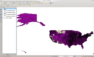
When finished, the file in PostGIS should look like this:

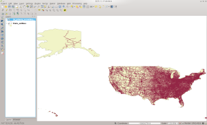
PRISECROADS in QGIS

Next we move on to the BG directory, which contains the state-based Census block groups.  Run lftp and mirror the BG directory.  Change to BG and run the unzip command that you did earlier to unzip all of the files into the same directory.  Then run the doogr.sh command in this directory and your output will look similar to the below:

[bmaddox@girls BG]$ doogr.sh us_census_bg.shp tl_2013_01_bg.shp
Creating initial state shapefile us_census_bg.shp
Now deleting the initial shapefiles to avoid duplication
Merging the rest of the files into the main shapefile
[bmaddox@girls BG]$ \rm tl*
[bmaddox@girls BG]$ ls -l
total 1074972
-rw-rw-r-- 1 bmaddox bmaddox 20970717 Mar 2 11:45 us_census_bg.dbf
-rw-rw-r-- 1 bmaddox bmaddox 165 Mar 2 11:45 us_census_bg.prj
-rw-rw-r-- 1 bmaddox bmaddox 1078018856 Mar 2 11:45 us_census_bg.shp
-rw-rw-r-- 1 bmaddox bmaddox 1766020 Mar 2 11:45 us_census_bg.shx
[bmaddox@girls BG]$

To add the now national-level Shapefile, run the following command:

[bmaddox@girls BG]$ shp2pgsql -s 4269 -c -D -I -WLATIN1 us_census_bg.shp US_Census_Block_Groups |psql -d Census_2013 
Shapefile type: Polygon
Postgis type: MULTIPOLYGON[2]
SET
SET
BEGIN
NOTICE: CREATE TABLE will create implicit sequence "us_census_block_groups_gid_seq" for serial column "us_census_block_groups.gid"
CREATE TABLE
NOTICE: ALTER TABLE / ADD PRIMARY KEY will create implicit index "us_census_block_groups_pkey" for table "us_census_block_groups"
ALTER TABLE
 addgeometrycolumn 
------------------------------------------------------------------------
 public.us_census_block_groups.geom SRID:4269 TYPE:MULTIPOLYGON DIMS:2 
(1 row)
CREATE INDEX
COMMIT
[bmaddox@girls BG]$

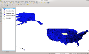
The data will look similar to this in QGIS:

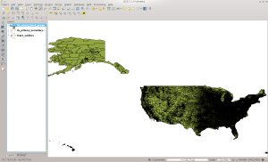
BG in QGIS

Next move on to the ELSD directory, that contains Elementary School Districts that the Census recognizes.  Again, run lftp and mirror the ELSD directory.  Then change into ELSD and run commands similar to below:

[bmaddox@girls ELSD]$ doogr.sh us_elsd.shp tl_2013_04_elsd.shp
Creating initial state shapefile us_elsd.shp
Now deleting the initial shapefiles to avoid duplication
Merging the rest of the files into the main shapefile
[bmaddox@girls ELSD]$ ls -l us_elsd.*
-rw-rw-r-- 1 bmaddox bmaddox 390701 Mar 2 12:17 us_elsd.dbf
-rw-rw-r-- 1 bmaddox bmaddox 165 Mar 2 12:17 us_elsd.prj
-rw-rw-r-- 1 bmaddox bmaddox 21617064 Mar 2 12:17 us_elsd.shp
-rw-rw-r-- 1 bmaddox bmaddox 17540 Mar 2 12:17 us_elsd.shx
[bmaddox@girls ELSD]$ shp2pgsql -s 4269 -c -D -I us_elsd.shp US_Elementary_School_Districts |psql -d Census_2013 
Shapefile type: Polygon
Postgis type: MULTIPOLYGON[2]
SET
SET
BEGIN
NOTICE: CREATE TABLE will create implicit sequence "us_elementary_school_districts_gid_seq" for serial column "us_elementary_school_districts.gid"
CREATE TABLE
NOTICE: ALTER TABLE / ADD PRIMARY KEY will create implicit index "us_elementary_school_districts_pkey" for table "us_elementary_school_districts"
ALTER TABLE
 addgeometrycolumn 
--------------------------------------------------------------------------------
 public.us_elementary_school_districts.geom SRID:4269 TYPE:MULTIPOLYGON DIMS:2 
(1 row)
CREATE INDEX
COMMIT
[bmaddox@girls ELSD]$

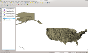
And this dataset will look like this in QGIS:

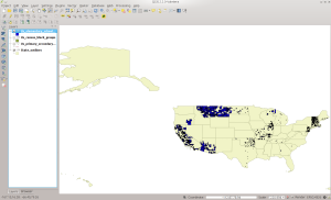
ELSD in QGIS

Moving on, now run lftp and mirror the SCSD and UNSD directories.  These are the Secondary School Districts and Unified School Districts, respectively.  Change to your SCSD directory and unzip all of the files there.  As you should be getting the hang of this now, here are the commands and their output once you have unzipped the tl* files.

[bmaddox@girls SCSD]$ doogr.sh us_scsd.shp tl_2013_04_scsd.shp
Creating initial state shapefile us_scsd.shp
Now deleting the initial shapefiles to avoid duplication
Merging the rest of the files into the main shapefile
[bmaddox@girls SCSD]$ ls -l us_scsd.*
-rw-rw-r-- 1 bmaddox bmaddox 93561 Mar 2 12:26 us_scsd.dbf
-rw-rw-r-- 1 bmaddox bmaddox 165 Mar 2 12:26 us_scsd.prj
-rw-rw-r-- 1 bmaddox bmaddox 10783856 Mar 2 12:26 us_scsd.shp
-rw-rw-r-- 1 bmaddox bmaddox 4260 Mar 2 12:26 us_scsd.shx
[bmaddox@girls SCSD]$ shp2pgsql -s 4269 -c -D -I -WLATIN1 us_scsd.shp US_Secondary_School_Districts |psql -d Census_2013 
Shapefile type: Polygon
Postgis type: MULTIPOLYGON[2]
SET
SET
BEGIN
NOTICE: CREATE TABLE will create implicit sequence "us_secondary_school_districts_gid_seq" for serial column "us_secondary_school_districts.gid"
CREATE TABLE
NOTICE: ALTER TABLE / ADD PRIMARY KEY will create implicit index "us_secondary_school_districts_pkey" for table "us_secondary_school_districts"
ALTER TABLE
 addgeometrycolumn 
-------------------------------------------------------------------------------
 public.us_secondary_school_districts.geom SRID:4269 TYPE:MULTIPOLYGON DIMS:2 
(1 row)
CREATE INDEX
COMMIT
[bmaddox@girls SCSD]$

And in QGIS:

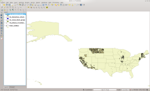
SCSD in QGIS

Next change to the UNSD directory, unzip the files, and run the commands as seen below:

[bmaddox@girls UNSD]$ doogr.sh us_unsd.shp tl_2013_01_unsd.shp
Creating initial state shapefile us_unsd.shp
Now deleting the initial shapefiles to avoid duplication
Merging the rest of the files into the main shapefile
[bmaddox@girls UNSD]$ \rm tl*
[bmaddox@girls UNSD]$ ls -l
total 216652
-rw-rw-r-- 1 bmaddox bmaddox 1958025 Mar 2 12:31 us_unsd.dbf
-rw-rw-r-- 1 bmaddox bmaddox 165 Mar 2 12:31 us_unsd.prj
-rw-rw-r-- 1 bmaddox bmaddox 219793844 Mar 2 12:31 us_unsd.shp
-rw-rw-r-- 1 bmaddox bmaddox 87588 Mar 2 12:31 us_unsd.shx
[bmaddox@girls UNSD]$ shp2pgsql -s 4269 -c -D -I -WLATIN1 us_unsd.shp US_Unified_School_Districts |psql -d Census_2013 
Shapefile type: Polygon
Postgis type: MULTIPOLYGON[2]
SET
SET
BEGIN
NOTICE: CREATE TABLE will create implicit sequence "us_unified_school_districts_gid_seq" for serial column "us_unified_school_districts.gid"
CREATE TABLE
NOTICE: ALTER TABLE / ADD PRIMARY KEY will create implicit index "us_unified_school_districts_pkey" for table "us_unified_school_districts"
ALTER TABLE
 addgeometrycolumn 
-----------------------------------------------------------------------------
 public.us_unified_school_districts.geom SRID:4269 TYPE:MULTIPOLYGON DIMS:2 
(1 row)
CREATE INDEX
COMMIT
[bmaddox@girls UNSD]$

And in QGIS:

UNSD in QGIS

Next, run lftp and mirror the SLDL and SLDU directories.  These are the State Legislative District Lower and Upper datasets.  Go into SLDL, unzip the files, and run these commands:

[bmaddox@girls SLDL]$ doogr.sh us_sldl.shp tl_2013_01_sldl.shp
Creating initial state shapefile us_sldl.shp
Now deleting the initial shapefiles to avoid duplication
Merging the rest of the files into the main shapefile
[bmaddox@girls SLDL]$ \rm tl*
[bmaddox@girls SLDL]$ ls -l
total 210476
-rw-rw-r-- 1 bmaddox bmaddox 841533 Mar 2 12:39 us_sldl.dbf
-rw-rw-r-- 1 bmaddox bmaddox 165 Mar 2 12:39 us_sldl.prj
-rw-rw-r-- 1 bmaddox bmaddox 214636500 Mar 2 12:39 us_sldl.shp
-rw-rw-r-- 1 bmaddox bmaddox 38772 Mar 2 12:39 us_sldl.shx
[bmaddox@girls SLDL]$ shp2pgsql -s 4269 -c -D -I -WLATIN1 us_sldl.shp US_State_Legislative_Lower |psql -d Census_2013 
Shapefile type: Polygon
Postgis type: MULTIPOLYGON[2]
SET
SET
BEGIN
NOTICE: CREATE TABLE will create implicit sequence "us_state_legislative_lower_gid_seq" for serial column "us_state_legislative_lower.gid"
CREATE TABLE
NOTICE: ALTER TABLE / ADD PRIMARY KEY will create implicit index "us_state_legislative_lower_pkey" for table "us_state_legislative_lower"
ALTER TABLE
 addgeometrycolumn 
----------------------------------------------------------------------------
 public.us_state_legislative_lower.geom SRID:4269 TYPE:MULTIPOLYGON DIMS:2 
(1 row)
CREATE INDEX
COMMIT
[bmaddox@girls SLDL]$

And in QGIS:

SLDL in QGIS

BTW, something did not go wrong if you notice that there is no data for Nebraska.  It has a unicameral form of government, which means it is not split into a House and Senate.

Next, change to the SLDU directory, unzip the files, and run the following commands:

[bmaddox@girls SLDU]$ doogr.sh us_sldu.shp tl_2013_01_sldu.shp
Creating initial state shapefile us_sldu.shp
Now deleting the initial shapefiles to avoid duplication
Merging the rest of the files into the main shapefile
[bmaddox@girls SLDU]$ shp2pgsql -s 4269 -c -D -I -WLATIN1 us_sldu.shp US_State_Legislative_Upper |psql -d Census_2013 
Shapefile type: Polygon
Postgis type: MULTIPOLYGON[2]
SET
SET
BEGIN
NOTICE: CREATE TABLE will create implicit sequence "us_state_legislative_upper_gid_seq" for serial column "us_state_legislative_upper.gid"
CREATE TABLE
NOTICE: ALTER TABLE / ADD PRIMARY KEY will create implicit index "us_state_legislative_upper_pkey" for table "us_state_legislative_upper"
ALTER TABLE
 addgeometrycolumn 
----------------------------------------------------------------------------
 public.us_state_legislative_upper.geom SRID:4269 TYPE:MULTIPOLYGON DIMS:2 
(1 row)
CREATE INDEX
COMMIT
[bmaddox@girls SLDU]$

And in QGIS:

SLDU in QGIS

I’m going to end this now so it is not as crazy long as the previous post was.  Next time we will work on the biggies of the Census datasets: roads, linearwater, areawater, and landmarks.