I’ve updated my datasets to the 2018 release of the Census Tiger Data. You can find them here.
Tiger 2018 Data Uploaded
Reply

I’ve updated my datasets to the 2018 release of the Census Tiger Data. You can find them here.
My first professional job during and after college was working at the US Geological Survey as a software engineer and researcher. My job required me to learn about GIS and cartography, as I would do things from writing production systems to researching distributed processing. It gave me an appreciation of cartography and of geospatial data. I especially liked topographic maps as they showed features such as caves and other interesting items on the landscape.
Recently, I had a reason to go back and recreate my mosaics of some Historic USGS Topomaps. I had originally put them into a PostGIS raster database, but over time realized that tools like QGIS and PostGIS raster can be extremely touchy when used together. Even after multiple iterations of trying out various overview levels and constraints, I still had issues with QGIS crashing or performing very slowly. I thought I would share my workflow in taking these maps, mosaicing them, and finally optimizing them for loading into a GIS application such as QGIS. Note that I use Linux and leave how to install the prerequisite software as an exercise for the reader.
As a refresher, the USGS has been scanning in old topographic maps and has made them freely available in GeoPDF format here. These maps are available at various scales and go back to the late 1800s. Looking at them shows the progression of the early days of USGS map making to the more modern maps that served as the basis of the USGS DRG program. As some of these maps are over one-hundred years old, the quality of the maps in the GeoPDF files can vary widely. Some can be hard to make out due to the yellowing of the paper, while others have tears and pieces missing.
Historically, the topographic maps were printed using multiple techniques from offset lithographic printing to Mylar separates. People used to etch these separates over light tables back in the map factory days. Each separate would represent certain parts of the map, such as the black features, green features, and so on. While at the USGS, many of my coworkers still had their old tool kits they used before moving to digital. You can find a PDF here that talks about the separates and how they were printed. This method of printing will actually be important later on in this series when I describe why some maps look a certain way.
Process
There are a few different ways to start out downloading USGS historic maps. My preferred method is to start at the USGS Historic Topomaps site.

USGS Historic Maps Search
It is not quite as fancy a web interface as the others, but it makes it easier to load the search results into Pandas later to filter and download. For my case, I was working on the state of Virginia, so I selected Virginia with a scale of 250,000 and Historical in the Map Type option. I purposely left Map Name empty and will demonstrate why later.
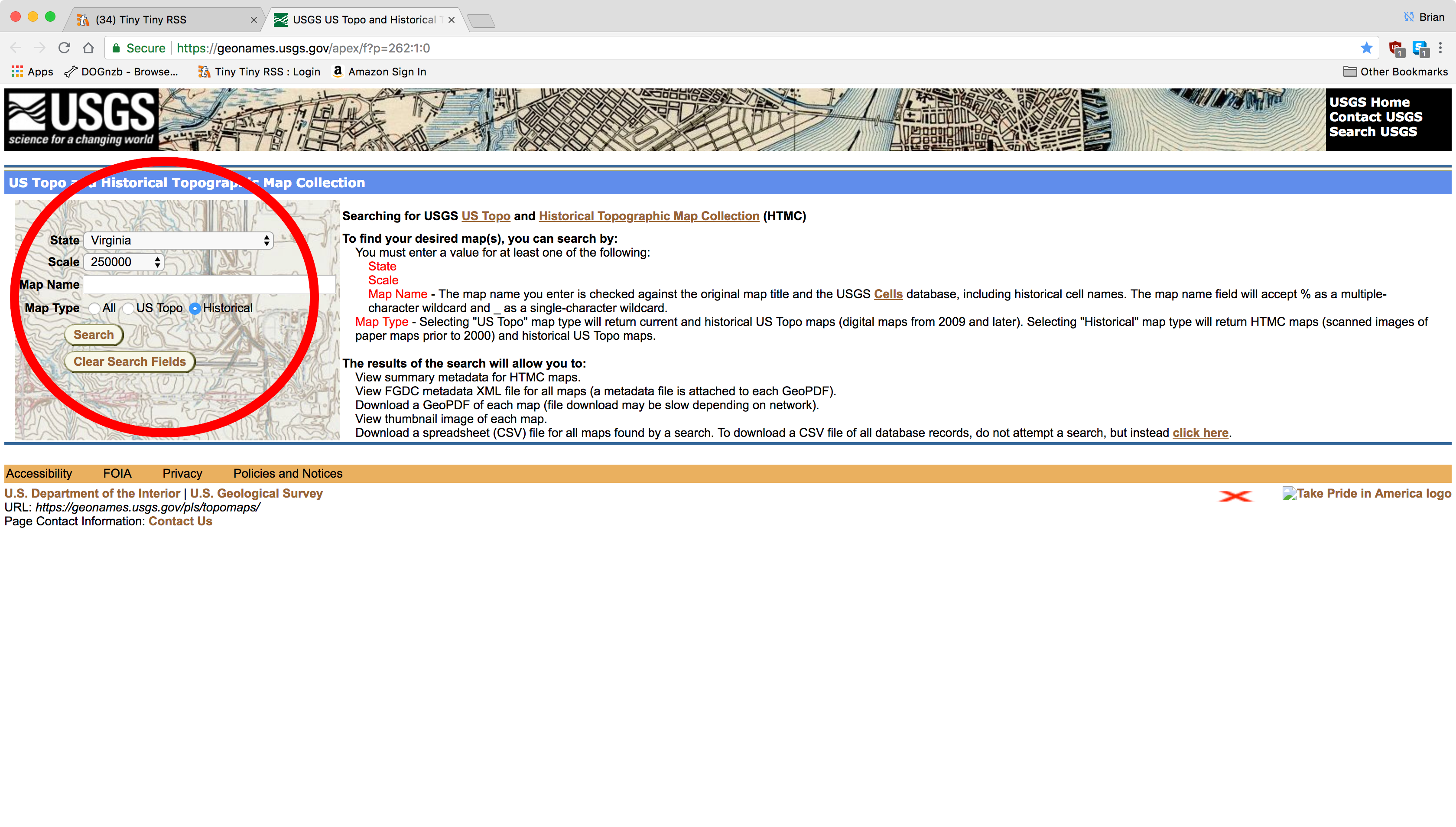
Topo Map Search
Once you click submit, you will see your list of results. They are presented in a grid view with metadata about each map that fits the search criteria. In this example case, there are eighty-nine results for 250K scale historic maps. The reason I selected this version of the search is that you can download the search results in a CSV format by clicking in the upper-right corner of the grid.

Topo Map Search Results
After clicking Download to Excel (csv) File, your browser will download a file called topomaps.csv. You can open it and see that there is quite a bit of metadata about each map.

Topo Map CSV Results
If you scroll to the right, you will find the column we are interested in called Download GeoPDF. This column contains the download URL for each file in the search results.

Highlighted CSV Column
For the next step, I rely on Pandas. If you have not heard of it, Pandas is an awesome Python data-analysis library that, among a long list of features, lets you load and manipulate a CSV easily. I usually load it using ipython using the commands in bold below.
bmaddox@sdf1:/mnt/filestore/temp/blog$ ipython3
Python 3.6.6 (default, Sep 12 2018, 18:26:19)
Type "copyright", "credits" or "license" for more information.

IPython 5.5.0 -- An enhanced Interactive Python.
?         -> Introduction and overview of IPython's features.
%quickref -> Quick reference.
help      -> Python's own help system.
object?   -> Details about 'object', use 'object??' for extra details.

In [1]: import pandas as pd

In [2]: csv = pd.read_csv("topomaps.csv")

In [3]: csv
Out[3]:
   Series     Version  Cell ID     ...      Scan ID GDA Item ID  Create Date
0    HTMC  Historical    69087     ...       255916     5389860   08/31/2011
1    HTMC  Historical    69087     ...       257785     5389864   08/31/2011
2    HTMC  Historical    69087     ...       257786     5389866   08/31/2011
3    HTMC  Historical    69087     ...       707671     5389876   08/31/2011
4    HTMC  Historical    69087     ...       257791     5389874   08/31/2011
5    HTMC  Historical    69087     ...       257790     5389872   08/31/2011
6    HTMC  Historical    69087     ...       257789     5389870   08/31/2011
7    HTMC  Historical    69087     ...       257787     5389868   08/31/2011
..    ...         ...      ...     ...          ...         ...          ...
81   HTMC  Historical    74983     ...       189262     5304224   08/08/2011
82   HTMC  Historical    74983     ...       189260     5304222   08/08/2011
83   HTMC  Historical    74983     ...       707552     5638435   04/23/2012
84   HTMC  Historical    74983     ...       707551     5638433   04/23/2012
85   HTMC  Historical    68682     ...       254032     5416182   09/06/2011
86   HTMC  Historical    68682     ...       254033     5416184   09/06/2011
87   HTMC  Historical    68682     ...       701712     5416186   09/06/2011
88   HTMC  Historical    68682     ...       701713     5416188   09/06/2011

[89 rows x 56 columns]

In [4]:
As you can see from the above, Pandas loads the CSV in memory along with the column names from the CSV header.
In [6]: csv.columns
Out[6]:
Index(['Series', 'Version', 'Cell ID', 'Map Name', 'Primary State', 'Scale',
       'Date On Map', 'Imprint Year', 'Woodland Tint', 'Visual Version Number',
       'Photo Inspection Year', 'Photo Revision Year', 'Aerial Photo Year',
       'Edit Year', 'Field Check Year', 'Survey Year', 'Datum', 'Projection',
       'Advance', 'Preliminary', 'Provisional', 'Interim', 'Planimetric',
       'Special Printing', 'Special Map', 'Shaded Relief', 'Orthophoto',
       'Pub USGS', 'Pub Army Corps Eng', 'Pub Army Map', 'Pub Forest Serv',
       'Pub Military Other', 'Pub Reclamation', 'Pub War Dept',
       'Pub Bur Land Mgmt', 'Pub Natl Park Serv', 'Pub Indian Affairs',
       'Pub EPA', 'Pub Tenn Valley Auth', 'Pub US Commerce', 'Keywords',
       'Map Language', 'Scanner Resolution', 'Cell Name', 'Primary State Name',
       'N Lat', 'W Long', 'S Lat', 'E Long', 'Link to HTMC Metadata',
       'Download GeoPDF', 'View FGDC Metadata XML', 'View Thumbnail Image',
       'Scan ID', 'GDA Item ID', 'Create Date'],
      dtype='object')
The column we are interested in is named Download GeoPDF as it contains the URLs to download the files.
In [7]: csv["Download GeoPDF"]
Out[7]:
0     https://prd-tnm.s3.amazonaws.com/StagedProduct...
1     https://prd-tnm.s3.amazonaws.com/StagedProduct...
2     https://prd-tnm.s3.amazonaws.com/StagedProduct...
3     https://prd-tnm.s3.amazonaws.com/StagedProduct...
4     https://prd-tnm.s3.amazonaws.com/StagedProduct...
5     https://prd-tnm.s3.amazonaws.com/StagedProduct...
6     https://prd-tnm.s3.amazonaws.com/StagedProduct...
7     https://prd-tnm.s3.amazonaws.com/StagedProduct...
                            ...
78    https://prd-tnm.s3.amazonaws.com/StagedProduct...
79    https://prd-tnm.s3.amazonaws.com/StagedProduct...
80    https://prd-tnm.s3.amazonaws.com/StagedProduct...
81    https://prd-tnm.s3.amazonaws.com/StagedProduct...
82    https://prd-tnm.s3.amazonaws.com/StagedProduct...
83    https://prd-tnm.s3.amazonaws.com/StagedProduct...
84    https://prd-tnm.s3.amazonaws.com/StagedProduct...
85    https://prd-tnm.s3.amazonaws.com/StagedProduct...
86    https://prd-tnm.s3.amazonaws.com/StagedProduct...
87    https://prd-tnm.s3.amazonaws.com/StagedProduct...
88    https://prd-tnm.s3.amazonaws.com/StagedProduct...
Name: Download GeoPDF, Length: 89, dtype: object
The reason I use Pandas for this step is that it gives me a simple and easy way to extract the URL column to a text file.
In [9]: csv["Download GeoPDF"].to_csv('urls.txt', header=None, index=None)
This gives me a simple text file that has all of the URLs in it.
https://prd-tnm.s3.amazonaws.com/StagedProducts/Maps/HistoricalTopo/PDF/DC/250000/DC_Washington_255916_1989_250000_geo.pdf
https://prd-tnm.s3.amazonaws.com/StagedProducts/Maps/HistoricalTopo/PDF/DC/250000/DC_Washington_257785_1961_250000_geo.pdf
https://prd-tnm.s3.amazonaws.com/StagedProducts/Maps/HistoricalTopo/PDF/DC/250000/DC_Washington_257786_1961_250000_geo.pdf
…
https://prd-tnm.s3.amazonaws.com/StagedProducts/Maps/HistoricalTopo/PDF/WV/250000/WV_Bluefield_254032_1961_250000_geo.pdf
https://prd-tnm.s3.amazonaws.com/StagedProducts/Maps/HistoricalTopo/PDF/WV/250000/WV_Bluefield_254033_1957_250000_geo.pdf
https://prd-tnm.s3.amazonaws.com/StagedProducts/Maps/HistoricalTopo/PDF/WV/250000/WV_Bluefield_701712_1957_250000_geo.pdf
https://prd-tnm.s3.amazonaws.com/StagedProducts/Maps/HistoricalTopo/PDF/WV/250000/WV_Bluefield_701713_1955_250000_geo.pdf
Finally, as there are usually multiple GeoPDF files that cover the same area, I download all of them so that I can go through and pick the best ones for my purposes. I try to find maps that are around the same data, are easily viewable, are not missing sections, and so on. To do this, I use the wget command and use the text file I created as input like so.
bmaddox@sdf1:/mnt/filestore/temp/blog$ wget -i urls.txt
--2018-09-23 13:00:41--  https://prd-tnm.s3.amazonaws.com/StagedProducts/Maps/HistoricalTopo/PDF/DC/250000/DC_Washington_255916_1989_250000_geo.pdf
Resolving prd-tnm.s3.amazonaws.com (prd-tnm.s3.amazonaws.com)... 52.218.194.10
Connecting to prd-tnm.s3.amazonaws.com (prd-tnm.s3.amazonaws.com)|52.218.194.10|:443... connected.
HTTP request sent, awaiting response... 200 OK
Length: 32062085 (31M) [application/pdf]
Saving to: ‘DC_Washington_255916_1989_250000_geo.pdf’
…
…
Eventually wget will download all the files to the same directory as the text file. In the next installment, I will continue my workflow as I produce mosaic state maps using the historic topographic GeoPDFs.
At my day job I am working on some natural language processing and need to generate a list of place names so I can further train the excellent spacy library. I previously imported the full Planet OSM so went there to pull a list of places. However, the place names in OSM are typically in the language of the person who did the collection, so they can be anything from English to Arabic. I stored the OSM data using imposm3 and included a PostgreSQL hstore column to store all of the user tags so we would not lose any data. I did a search for all tags that had values like name and en in them and exported those keys and values to several CSV files based on the points, lines, and polygons tables. I thought I would write a quick post to show how easy it can be to manipulate data outside of traditional spreadsheet software.
The next thing I needed to do was some data reduction, so I went to my go-to library of Pandas. If you have been living under a rock and have not heard of it, Pandas is an exceptional data processing library that allows you to easily manipulate data from Python. In this case, I knew some of my data rows were empty and that I would have duplicates due to how things get named in OSM. Pandas makes cleaning data incredibly easy in this case.
First I needed to load the files into Pandas to being cleaning things up. My personal preference for a Python interpreter is ipython/jupyter in a console window. To do this I ran ipython and then imported Pandas by doing the following:
In [1]: import pandas as pd
Next I needed to load up the CSV into Pandas to start manipulating the data.
In [2]: df = pd.read_csv('osm_place_lines.csv', low_memory=False)
At this point, I could examine how many columns and rows I have by running:
In [3]: df.shape
Out[3]: (611092, 20)
Here we can see that I have 611,092 rows and 20 columns. My original query pulled a lot of columns because I wanted to try to capture as many pre-translated English names as I could. To see what all of the column names are, I just had to run:
In [10]: df.columns
Out[10]:
Index(['name', 'alt_name_1_en', 'alt_name_en', 'alt_name_en_2',
       'alt_name_en_3', 'alt_name_en_translation', 'en_name',
       'gns_n_eng_full_name', 'name_en', 'name_ena', 'name_en1', 'name_en2',
       'name_en3', 'name_en4', 'name_en5', 'name_en6', 'nam_en', 'nat_name_en',
       'official_name_en', 'place_name_en'],
      dtype='object')
The first task I then wanted to do was drop any rows that had no values in them. In Pandas, empty cells default to the NaN value. So to drop all the empty rows, I just had to run:
In [4]: df = df.dropna(how='all')
To see how many rows fell out, I again checked the shape of the data.
In [5]: df.shape
Out[5]: (259564, 20)
Here we can see that the CSV had 351,528 empty rows where the line had no name or English name translations.
Next, I assumed that I had some duplicates in the data. Some things in OSM get generic names, so these can be filtered out since I only want the first row from each duplicate. With no options, drop_duplicates() in Pandas only keeps the first value.
In [6]: df = df.drop_duplicates()
Checking the shape again, I can see that I had 68,131 rows of duplicated data.
In [7]: df.shape
Out[7]: (191433, 20)
At this point I was interested in how many cells in each row still contained no data. The CSV was already sparse since I converted each hstore key into a separate column in my output. To do this, I ran:
In [8]: df.isna().sum()
Out[8]:
name                          188
alt_name_1_en              191432
alt_name_en                190310
alt_name_en_2              191432
alt_name_en_3              191432
alt_name_en_translation    191432
en_name                    191430
gns_n_eng_full_name        191432
name_en                    191430
name_ena                   172805
name_en1                   191409
name_en2                   191423
name_en3                   191429
name_en4                   191430
name_en5                   191432
name_en6                   191432
nam_en                     191432
nat_name_en                191431
official_name_en           191427
place_name_en              191429
dtype: int64
Here we can see the sparseness of the data. Considering I am now down to 191,433 columns, some of the columns only have a single entry in them. We can also see that I am probably not going to have a lot of English translations to work with.
At this point I wanted to save the modified dataset so I would not loose it. This was a simple
In [8]: df.to_csv('osm_place_lines_nonull.csv', index=False)
The index=False option tells Pandas to not output its internal index field to the CSV.
Now I was curious what things looked like, so I decided to check out the name column. First I increased some default values in Pandas because I did not want it to abbreviate rows or columns.
pd.set_option('display.max_rows', 200)
pd.set_option('display.max_columns', 25)
To view the whole row where the value in a specific column is null, I did the following and I will abbreviate the output to keep the blog shorter 🙂
df[df['name'].isnull()]
...
       name_en                                 name_ena name_en1 name_en2  \
166        NaN                        Orlovskogo Island      NaN      NaN
129815     NaN                            Puukii Island      NaN      NaN
159327     NaN                           Ometepe Island      NaN      NaN
162420     NaN                                  Tortuga      NaN      NaN
164834     NaN                         Jack Adan Island      NaN      NaN
191664     NaN                            Hay Felistine      NaN      NaN
193854     NaN             Alborán Island Military Base      NaN      NaN
197893     NaN                         Carabelos Island      NaN      NaN
219472     NaN                           Little Fastnet      NaN      NaN
219473     NaN                             Fastnet Rock      NaN      NaN
220004     NaN                           Doonmanus Rock      NaN      NaN
220945     NaN                             Tootoge Rock      NaN      NaN
229446     NaN                               Achallader      NaN      NaN
238355     NaN                            Ulwile Island      NaN      NaN
238368     NaN                             Mvuna Island      NaN      NaN
238369     NaN                            Lupita Island      NaN      NaN
238370     NaN                              Mvuna Rocks      NaN      NaN
259080     NaN                                  Kafouri      NaN      NaN
259235     NaN                              Al Thawra 8      NaN      NaN
259256     NaN                              Beit al-Mal      NaN      NaN
261584     NaN                                   Al Fao      NaN      NaN
262200     NaN                                  May 1st      NaN      NaN
...
Now that I have an idea how things look, I can do things like fill out the rest of the name columns with the English names found the various other columns.
As I’ve posted before, the download from the USGS Geonames site has some problems. The feature_id column should be unique, but it is not because the file contains some of the same feature names in Mexico and Canada with the same id which breaks the unique constraint.
I just added a very quick and dirty python program to my misc_gis_scripts repo on Github. It’s run by
python3 gnisfixer.py downloadedgnisfile newgnisfile
For the latest download, it removed over 7,000 non-US or US Territory entries and into the DB perfectly.
Since I needed it as part of my job, I finally got around to finishing up the Geonames scripts in my github repository misc_gis_scripts. In the geonames subdirectory is a bash script called dogeonames.sh. Create a PostGIS database, edit the bash file, and then run it and it will download and populate your Geonames database for you.
Note that I’m not using the alternatenamesv2 file that they’re distributing now. I checked with a hex editor and they’re not actually including all fields on each line, and Postgres will not import a file unless each column is there. I’ll probably add in a Python file to fix it at some point but not now 🙂
I just uploaded all of the 2017 US Census Tiger datasets where I’ve converted them from county-based to state-based ShapeFiles. You can find them in my GIS Data section. Let me know of any errors you come across. Note I haven’t done all of the Census data, just the ones I regularly use.
A while back I picked up a Raspberry Pi 3 and turned it into a NAS and LAMP stack server (Apache, PostgreSQL, Mysql, PostGIS, and so on). Later I came across forums mentioning a new entry from Asus into this space called the Tinkerboard. Now I’m not going to go into an in-depth review since you can find those all over the Internet. However, I do want to mention a few things I’ve found and done that are very helpful. I like the board since it’s supports things like OpenCL and pound for pound is more powerful than the Pi 3. The two gig of RAM vs one with the Pi 3 makes it useful for more advanced processing.
One thing to keep in mind is that the board is still “new” and has a growing community. As such there are going to be some pains, such as not having as big a community as the Pi ecosystem. But things do appear to be getting better, and so far it’s proven to be more capable and, in some cases, more stable than my Pi 3.
So without much fanfare, here are my list of tips for using the Tinkerboard. You can find a lot more information online.
I’ll have more to say about this board later.
When I went to import the latest GNIS dataset into my local PostGIS database, I found that it contains the same issues I’ve been reporting for the past few years. You can find my fixed version of the dataset here.
As a disclaimer, while I used to work there, I no longer have any association with the US Geological Survey or the Board of Geographic Names.
For those interested, here is the list of problems I found and fixed:
ID 45605: Duplicate entry for Parker Canyon, AZ. The coordinates are in Sonora, Mexico.
ID 45606: Duplicate entry for San Antonio Canyon, AZ. The coordinates are in Sonora, Mexico.
ID 45608: Duplicate entry for Silver Creek, AZ. The coordinates are in Sonora, Mexico.
ID 45610: Duplicate entry for Sycamore Canyon, AZ. The coordinates are in Sonora, Mexico.
ID 567773: Duplicate entry for Hovey Hill, ME. The coordinates are in New Brunswick, Canada.
ID 581558: Duplicate entry for Saint John River, ME. The coordinates are in New Brunswick, Canada.
ID 768593: Duplicate entry for Bear Gulch, MT.  The coordinates are in Alberta, Canada.
ID 774267: Duplicate entry for Miners Coulee, MT.  The coordinates are in Alberta, Canada.
ID 774784: Duplicate entry for North Fork Milk River, MT.  The coordinates are in Alberta, Canada.
ID 775339: Duplicate entry for Police Creek, MT.  The coordinates are in Alberta, Canada.
ID 776125: Duplicate entry for Saint Mary River, MT.  The coordinates are in Alberta, Canada.
ID 778142: Duplicate entry for Waterton River, MT.  The coordinates are in Alberta, Canada.
ID 778545: Duplicate entry for Willow Creek, MT.  The coordinates are in Alberta, Canada.
ID 798995: Duplicate entry for Lee Creek, MT.  The coordinates are in Alberta, Canada.
ID 790166: Duplicate entry for Screw Creek, MT.  The coordinates are in British Columbia, Canada.
ID 793276: Duplicate entry for Wigwam River, MT.  The coordinates are in British Columbia, Canada.
ID 1504446: Duplicate entry for Depot Creek, WA.  The coordinates are in British Columbia, Canada.
ID 1515954: Duplicate entry for Arnold Slough, WA.  The coordinates are in British Columbia, Canada.
ID 1515973: Duplicate entry for Ashnola River, WA.  The coordinates are in British Columbia, Canada.
ID 1516047: Duplicate entry for Baker Creek, WA.  The coordinates are in British Columbia, Canada.
ID 1517465: Duplicate entry for Castle Creek, WA.  The coordinates are in British Columbia, Canada.
ID 1517496: Duplicate entry for Cathedral Fork, WA.  The coordinates are in British Columbia, Canada.
ID 1517707: Duplicate entry for Chilliwack River, WA.  The coordinates are in British Columbia, Canada.
ID 1517762: Duplicate entry for Chuchuwanteen Creek, WA.  The coordinates are in British Columbia, Canada.
ID 1519414: Duplicate entry for Ewart Creek, WA. The coordinates are in British Columbia, Canada.
ID 1520446: Duplicate entry for Haig Creek, WA. The coordinates are in British Columbia, Canada.
ID 1520654: Duplicate entry for Heather Creek, WA. The coordinates are in British Columbia, Canada.
ID 1521214: Duplicate entry for International Creek, WA. The coordinates are in British Columbia, Canada.
ID 1523541: Duplicate entry for Myers Creek, WA. The coordinates are in British Columbia, Canada.
ID 1523731: Duplicate entry for North Creek, WA. The coordinates are in British Columbia, Canada.
ID 1524131: Duplicate entry for Pack Creek, WA. The coordinates are in British Columbia, Canada.
ID 1524235: Duplicate entry for Pass Creek, WA. The coordinates are in British Columbia, Canada.
ID 1524303: Duplicate entry for Peeve Creek, WA. The coordinates are in British Columbia, Canada.
ID 1525297: Duplicate entry for Russian Creek, WA. The coordinates are in British Columbia, Canada.
ID 1525320: Duplicate entry for Saar Creek, WA. The coordinates are in British Columbia, Canada.
ID 1527272: Duplicate entry for Togo Creek, WA. The coordinates are in British Columbia, Canada.
ID 1529904: Duplicate entry for McCoy Creek, WA. The coordinates are in British Columbia, Canada.
ID 1529905: Duplicate entry for Liumchen Creek, WA. The coordinates are in British Columbia, Canada.
ID 942345: Duplicate entry for Allen Brook, NY. The coordinates are in Quebec, Canada.
ID 949668: Duplicate entry for English River, NY. The coordinates are in Quebec, Canada.
ID 959094: Duplicate entry for Oak Creek, NY. The coordinates are in Quebec, Canada.
ID 967898: Duplicate entry for Trout River, NY. The coordinates are in Quebec, Canada.
ID 975764: Duplicate entry for Richelieu River, VT. The coordinates are in Quebec, Canada.
ID 1458184: Duplicate entry for Leavit Brook, VT. The coordinates are in Quebec, Canada.
ID 1458967: Duplicate entry for Pike River, VT. The coordinates are in Quebec, Canada.
ID 1028583: Duplicate entry for Cypress Creek, ND. The coordinates are in Manitoba, Canada.
ID 1035871: Duplicate entry for Mowbray Creek, ND. The coordinates are in Manitoba, Canada.
ID 1035887: Duplicate entry for Gimby Creek, ND. The coordinates are in Manitoba, Canada.
ID 1035890: Duplicate entry for Red River of the North, ND. The coordinates are in Manitoba, Canada.
ID 1035895: Duplicate entry for Wakopa Creek, ND. The coordinates are in Manitoba, Canada.
ID 1930555: Duplicate entry for Red River of the North, ND. The coordinates are in Manitoba, Canada.
ID 1035882: Duplicate entry for East Branch Short Creek, ND. The coordinates are in Saskatchewan, Canada.
ID 1782010: Duplicate entry for Manitoulin Basin, MI. The coordinates are in Ontario, Canada
So I have been meaning to finish up this series for a while now, but other things got in the way (which hopefully I can post on here soon). In the mean time, there are numerous tutorials on-line now about how to set a Pi up as a home file server, so I think I will defer to those instead of wasting more bits on the Internet. However, I would like to point out some things I have done that has resulted in my Pi setup being nice and stable.
This biggest thing to do when using the SD card as the root file system for the Pi is to minimize the number of writes to it. This will help keep it lasting longer and avoid any file system corruption. One thing you can do is modify your /etc/fstab and use the noatime family of attributes. The default of most Pi distributions is ext3/4, so this should work for you. First find your entry in the /etc/fstab for your /. In mine below, you can see it’s /dev/mmcblk0p2:
proc /proc proc defaults 0 0
/dev/mmcblk0p2 / ext4 defaults 0 1
/dev/mmcblk0p1 /boot/ vfat defaults 0 2
/dev/md0 /mnt/filestore xfs defaults,nofail 0 2
Change line 2 so that it reads like this:
/dev/mmcblk0p2 / ext4 defaults,noatime,nodiratime 0
This will stop the file system from modifying itself each time a directory or file is accessed.
As you can see from my fstab, I also have my RAID partition on the enclosure set to xfs and I use the nofail attribute. This is very important since your enclosure may not be fully spun up and ready by the time your Pi tries to mount it. If it’s not there, the Pi will hang (forever in my case since it will cause the kernel to panic).
I also run mariadb and postgresql with postgis on the Pi3, however I have them set to not autostart by running:
systemctl disable mysqld
systemctl disable postgresql
I could leave them running since I’ve lowered their memory requirements, but choose to only have things running on the Pi 3 whenever I need it to make sure I don’t run out of memory.
I put their respective data directories on the NAS and then made a soft link under /var by running;
ln -s /mnt/filestore/data/mysql /var/lib/mysql
ln -s /mnt/filestore/data/postgresql /var/lib/postgresql
You could edit their config files to change the location, but for me I have found it is easier to simply use soft links. Plus, since the servers are not set to start a boot, I do not have to worry about any errors every time the Pi restarts.
I also run recoll on the Pi as I have collected several hundred gigabytes of papers and ebooks over the years. Recoll is a nice utility that provides a semantic search ability. By default, recoll and run your file system and system itself into the ground if you let it. I made a few tweaks so that would play nice whenever I run it periodically on the Pi. The first thing I did was move the ~/.recoll directory to the NAS and create a soft link by running
ln -s /mnt/filestore/data recoll .recoll
Again, the goal is to reduce the number of file system access to the SD card itself. Secondly, I created the .recoll/recoll.conf file with the following contents:
topdirs = /mnt/filestore/data/Documents /mnt/filestore/data/ebooks /mnt/filestore/data/Programming
filtermaxseconds 60
thrQSizes = -1 -1 -1
The filtermaxseconds parameter tells recoll to stop indexing a file if the filter runs for a whole minute. The thrQSizes option has recoll use a single thread. While this makes it slower, it makes things run much better on the Pi while still allowing other services to run.
If you want to run other services, keep in mind that if they do a lot of I/O, you should move them to your external drive and use a soft link to redirect like I did above. Doing so will help to greatly extend the life of your SD card and keep you from having to reimage it.
In the last article, I went over my decisions about the hardware I wanted to use to build a cheap home NAS. Here I will go over the software and configuration to get everything working.
Once all the parts came in, it was time to get going and configure everything. First, though, I would like to talk about SD cards, and why I feel they are the one major flaw with the Raspberry Pi series.
Conceptually, SD cards are a great thing. They come in different sizes and can store multiple gigabytes of data on them. They are used in everything from cell phones to digital cameras to computers. You are probably using one daily in a device without even knowing it.
You might think there are hundreds of companies making them, and you would be wrong. See, as with many things, a few companies actually make the physical cards and then a lot of other companies will buy and re-brand them. The companies that slap their logo on these cards do not care whether they buy quality card stock as long as it is cheap. So what we end up with is a situation where you can by two of the same “type” of SD card and physically they could be quite different from each other.
You also may not realize that SD cards are just as capable of developing bad sectors as your physical hard drive is. Some cards have a smart enough controller built-in that will automatically remap bad sectors to other good spaces on the card like SMART does with hard drives. Many others do not and have a “dumb” controller that does the bare minimum to make the device work.
The reality with SD cards is that expecting them to “just work” is about as safe as playing Russian roulette with all six cylinders loaded. Just as with hard drives, your SD WILL fail. Unlike hard drives, your SD may or may not be able to take care of problems on its own. And with the wild west of the cards, well, your best bet is to never trust that data on them is safe.
At my previous job I spent a lot of time dealing with SD cards and learning how to deal with their various issues. Often we would have random problems come up that could not be explained, only to find out that the SD card had developed issues that needed to be corrected to return things to normal. What I found out after looking at the low level portions of the card and a lot of reading has made me rethink trusting these devices for long term storage and use. The Pi will be running an operating system off of the SD, so you can expect a lot of reads and writes being done to it. This will speed up the development of bad sectors on the device and reduce its operating lifetime.
There are a few things you can do to help things. Before you even start to install software for your Pi, I highly recommend that you do the check the physical surface of the SD before you use it, even if it is new out of the package. I’m writing this from a Linux perspective, but the same information applies to Windows or even Mac OS as well. As usual, your mileage may vary. Doing this could cause you to lose data and make dogs and cats live together in a dystopian future. This will take some extra time, but I firmly believe it is worth it.
Plug the SD into your computer and identify what device it is assigned. I will leave it up to you to web search this for bonus points. First thing I recommend is using the dd command to write random data to the entire device. If the SD card has an intelligent controller, this will help it to determine if there are any bad sectors and remap them before you put Linux on it for the Pi. Even without an intelligent controller, initially writing to it can help find spots that may be bad or trigger marginal sectors to go bad. Run a command similar to:
dd if=/dev/random of=/your/sd/device bs=8M
This command will write a random value to each byte on your SD card. Once this is done, the next thing I recommend is format the SD and check for bad sectors while formatting. This can be done with something along the lines of:
mkfs.ext4 -cc /your/sd/device
This command will put a file system on the SD and do a read/write test while formatting it. Along with the dd command, this should bang on the physical surface of the card enough to find any initial bad sectors that could already be there.
That is it for this installment. Now that my soapbox is over, next time we will talk installing software and configuring the Pi to be a NAS.