Here’s the first map I’ve done based on the GeoPDFs from the USGS Historic Map Collection.  I found all of the available maps for Virginia at the 125K scale and the vintages were from 1888 to 1902.  It’s a GeoTIFF that is 484M in size and compressed using LZW lossless compression.

Link to the map.

For this installment, we will look at importing data from OpenStreetMap.org.  As I mentioned in an earlier post, OpenStreetMap is a cloud-sourced GIS dataset with the goal of producing a global dataset that anyone can use.  There are two ways to download this data: you can either use Bittorrent and download the entire planet from http://osm-torrent.torres.voyager.hr/ or download extracts from http://download.geofabrik.de/.  If you do not need the entire planet, I would highly recommend using geofabrik.  It has a fast downlink and they have finally added MD5 checksums so you can verify the integrity of your download.

Go to http://download.geofabrik.de/ and click on North America.  We will be using the .pbf format file so click the link near the top of the page named north-america-latest.osm.pbf.  It is about six gigabytes in size and the MD5sum is listed at the end of the paragraph.  Once the download is done in your browser, you can use the md5sum command under a Linux shell or download one of the many MD5sum clients for windows.  It will look similar to the below example output (it likely will not match exactly as the MD5 value will change as the data is modified.

bmaddox@girls:~/Downloads/geodata$ md5sum north-america-latest.osm.pbf 
d2daa9c7d3ef4dead4a2b5f790523e6d north-america-latest.osm.pbf
bmaddox@girls:~/Downloads/geodata$

Next go back to the main geofabrik site and then click on and download the Central America file.  This will give you Mexico and the other Central American files.  As listed above, once the download is done in your browser, check it with md5sum.  If the values do not match, you will want to redownload and rerun md5sum again until they do.

There are several programs you can use to import OpenStreetMap data into PostGIS.  They mainly differ on what schema they use and how they manipulate the data before it goes in.  For purposes of this post, we will be using the imposm program found at http://imposm.org/docs/imposm/latest/.  If you are on Ubuntu, it should be a simple apt-get install imposm away.  For Windows or other distributions, you can download it directly from the imposm website.  The tutorial on how to import data using imposm can be found here: http://imposm.org/docs/imposm/latest/tutorial.html.

Using imposm is a multi-stage process.  The first stage is to have it read the data and combine the files into several intermediary files.  First create a PostGIS database by running:

createdb -T gistemplate OSM

Now have imposm take the data and convert it into its intermediary files.  To do this, run a similar command to this:

bmaddox@girls:/data/data/geo$ imposm --read --concurrency 2 --proj EPSG:4326 ~/Downloads/geodata/*.pbf
[16:29:15] ## reading /home/bmaddox/Downloads/geodata/central-america-latest.osm.pbf
[16:29:15] coords: 500489k nodes: 10009k ways: 71498k relations: 500k (estimated)
[16:31:27] coords: 21524k nodes: 92k ways: 2464k relations: 5k
[16:31:28] ## reading /home/bmaddox/Downloads/geodata/north-america-latest.osm.pbf
[16:31:28] coords: 500489k nodes: 10009k ways: 71498k relations: 500k (estimated)
[17:40:22] coords: 678992k nodes: 1347k ways: 44469k relations: 229k
[17:40:23] reading took 1 h 11m 7 s
[17:40:23] imposm took 1 h 11m 7 s
bmaddox@girls:/data/data/geo$

Here, I changed to a different drive and can the imposm command to read from the drive where I downloaded the .pbf files.  I did this since reading is a disk intensive process and spitting it between drives helps to speed things up a bit.  Also, I differed from the tutorial as my install of QGIS could not render OpenStreetMap data in its native EPSG:900913 projection with data in the EPSG:4326 coordinate system that my Tiger data was in.  Unless you have an extremely high-end workstation, this will take a while.  Once the process is done, you will have the following files in the output directory:

bmaddox@girls:~/Downloads/geodata/foo$ dir
imposm_coords.cache imposm_nodes.cache imposm_relations.cache imposm_ways.cache

The next step is to take the intermediary files and write them into PostGIS.  Here you can use a wild card to read all of the .pbf files you downloaded.

bmaddox@girls:~/Downloads/geodata/foo$ imposm --write --database OSM --host localhost --user bmaddox --port 5432 --proj EPSG:4326
password for bmaddox at localhost:
[18:20:21] ## dropping/creating tables
[18:20:22] ## writing data
[2014-06-15 18:52:46,074] imposm.multipolygon - WARNING - building relation 1834172 with 8971 ways (10854.8ms) and 8843 rings (2293.0ms) took 426854.5ms
[2014-06-15 19:00:47,635] imposm.multipolygon - WARNING - building relation 2566179 with 4026 ways (4717.3ms) and 3828 rings (1115.6ms) took 89522.6ms
[19:15:20] relations: 244k/244k
[19:15:41] relations: total time 55m 18s for 244095 (73/s)
[00:35:28] ways: 46907k/46907k
[00:35:30] ways: total time 5 h 19m 49s for 46907462 (2444/s)
[00:40:21] nodes: 1437k/1437k
[00:40:22] nodes: total time 4 m 51s for 1437951 (4933/s)
[00:40:22] ## creating generalized tables
[01:44:47] generalizing tables took 1 h 4 m 24s
[01:44:47] ## creating union views
[01:44:48] creating views took 0 s
[01:44:48] ## creating geometry indexes
[02:15:02] creating indexes took 30m 14s
[02:15:02] writing took 7 h 54m 41s
[02:15:02] imposm took 7 h 54m 42s
bmaddox@girls:~/Downloads/geodata/foo$

As you can see from the above output, this took almost eight hours on my home server (quad core AMD with eight gig of RAM).  This command loads all of the data from the intermediate files into PostGIS.  However, we are not done yet.  Looking at the output, all it did was load the data and create indices.  It did not cluster the data or perform any other optimizations.  To do this, run the following imposm command:

bmaddox@girls:~/Downloads/geodata/foo$ imposm --optimize -d OSM --user bmaddox
password for bmaddox at localhost:
[17:18:12] ## optimizing tables
Clustering table osm_new_transport_areas
Clustering table osm_new_mainroads
Clustering table osm_new_buildings
Clustering table osm_new_mainroads_gen1
Clustering table osm_new_mainroads_gen0
Clustering table osm_new_amenities
Clustering table osm_new_waterareas_gen1
Clustering table osm_new_waterareas_gen0
Clustering table osm_new_motorways_gen0
Clustering table osm_new_aeroways
Clustering table osm_new_motorways
Clustering table osm_new_transport_points
Clustering table osm_new_railways_gen0
Clustering table osm_new_railways_gen1
Clustering table osm_new_landusages
Clustering table osm_new_waterways
Clustering table osm_new_railways
Clustering table osm_new_motorways_gen1
Clustering table osm_new_waterareas
Clustering table osm_new_places
Clustering table osm_new_admin
Clustering table osm_new_minorroads
Clustering table osm_new_landusages_gen1
Clustering table osm_new_landusages_gen0
Vacuum analyze
[19:24:38] optimizing took 2 h 6 m 25s
[19:24:38] imposm took 2 h 6 m 26s
bmaddox@girls:~/Downloads/geodata/foo$

On my system it took a couple of hours and clustered all of the tables and then did a vacuum analyze to update the database statistics.

The final step is to have imposm rename the tables to what they will be in “production mode”.  Run the following:

bmaddox@girls:~/Downloads/geodata/foo$ imposm -d OSM --user bmaddox --deploy-production-tables
password for bmaddox at localhost:
[11:00:06] imposm took 1 s
bmaddox@girls:~/Downloads/geodata/foo$

Your data should now be optimized and ready for use.  To test it, refer to an earlier post in this series where I discussed using QGIS and load some of the OSM data into it.

Your OSM database will have the following tables in it:

 List of relations
 Schema | Name | Type | Owner 
--------+----------------------+-------+---------
 public | osm_admin | table | bmaddox
 public | osm_aeroways | table | bmaddox
 public | osm_amenities | table | bmaddox
 public | osm_buildings | table | bmaddox
 public | osm_landusages | table | bmaddox
 public | osm_landusages_gen0 | table | bmaddox
 public | osm_landusages_gen1 | table | bmaddox
 public | osm_mainroads | table | bmaddox
 public | osm_mainroads_gen0 | table | bmaddox
 public | osm_mainroads_gen1 | table | bmaddox
 public | osm_minorroads | table | bmaddox
 public | osm_motorways | table | bmaddox
 public | osm_motorways_gen0 | table | bmaddox
 public | osm_motorways_gen1 | table | bmaddox
 public | osm_places | table | bmaddox
 public | osm_railways | table | bmaddox
 public | osm_railways_gen0 | table | bmaddox
 public | osm_railways_gen1 | table | bmaddox
 public | osm_transport_areas | table | bmaddox
 public | osm_transport_points | table | bmaddox
 public | osm_waterareas | table | bmaddox
 public | osm_waterareas_gen0 | table | bmaddox
 public | osm_waterareas_gen1 | table | bmaddox
 public | osm_waterways | table | bmaddox
 public | spatial_ref_sys | table | bmaddox
(25 rows)

The _gen0 and _gen1 tables are generalized and not as highly detailed as the other tables.  They are good for viewing data over large geographic areas (think nation scale).  With areas that large, it would take a lot of time to render the high resolution data.  Thus the _gen0 and _gen1 tables are simplified versions of the data for use at these resolutions.  You can use QGIS’s scale-dependent rendering to specify these tables and then go to the high-resolution tables upon zooming in.

Go forth and play with the additional free geospatial data you now have in your database 🙂

Updated 23 March 2018: Changed for new size necessary for the cc2 column

It’s been a while since I’ve made a post, so thought I’d keep going with the data series.  This time around I’ll be talking about how to make your own local copy of the NGA Geonames database.  This database is similar to GNIS, but covers the whole globe and also has information on location such as airfields, pipelines, and so on.

First, download the following files from the Geonames website:

• admin1CodesASCII.txt
• admin2Codes.txt
• allCountries.txt
• alternateNamesV2.txt
• countryInfo.txt
• featureCodes_en.txt
• hierarchy.txt
• iso-languagecodes.txt
• timeZones.txt
• userTags.txt

Some of them are zipped, so you’ll need to unzip them into the same directory as the others for ease of use.  Next, create your geonames database by running:

bmaddox@girls:~/Downloads/geodata$ createdb -T gistemplate Geonames

Next, we will create the table for the main points file, which is called allCountries.txt.  Run the following command from the same directory where you have all of the Geonames files:

bmaddox@girls:~/Downloads/geodata$ psql -d Geonames 
psql (9.3.4)
Type "help" for help.
Geonames=#

This will put you into the PostgreSQL command line.  Now create the table to hold the data in the allCountries.txt file:

Geonames=# create table geoname (
geonameid int,
name varchar(200),
asciiname varchar(200),
alternatenames text,
latitude float,
longitude float,
fclass char(1),
fcode varchar(10),
country varchar(2),
cc2 varchar(170),
admin1 varchar(20),
admin2 varchar(80),
admin3 varchar(20),
admin4 varchar(20),
population bigint,
elevation int,
dem int,
timezone varchar(40),
moddate date
);
CREATE TABLE
Geonames=#

Now we will use a built-in PostgreSQL command to load data in the DB.  There are two forms of it, the long way specifies the column names in order on the command line, the other just the file name.  We will be using the short way here:

Geonames=# \copy geoname from allCountries.txt null as '';
Geonames=#

This loads the data, but it is not yet ready to be usable by a GIS.  We will need to create a geometry column for the data and then use the latitude and longitude columns to create a point column in the geometry.

Geonames=# SELECT AddGeometryColumn( 'geoname', 'the_geom', 4326, 'POINT', 2);
 addgeometrycolumn 
------------------------------------------------------
 public.geoname.the_geom SRID:4326 TYPE:POINT DIMS:2 
(1 row)
Geonames=#

This command creates the geometry column, and specifies an EPSG of 4326 (WGS84).  Now we need to insert the latitude and longitudes of the points into this column:

Geonames=# update geoname SET the_geom = ST_PointFromText('POINT(' || longitude || ' ' || latitude || ')', 4326);
UPDATE 8943136
Geonames=#

This will take a while as PostGIS must read each point, convert it into the proper format, and then add it into the geometry column.  Now we need to add a geospatial index on this column to make the queries faster.  Again, it may take a while to run.

Geonames=# create index geoname_the_geom_gist_idx on geoname using gist (the_geom);
CREATE INDEX
Geonames=#

Once this is done, we should optimize this table as I mentioned in a previous post.  We need to analyze the database and then cluster it on the points.

Geonames=# vacuum analyze geoname;
VACUUM
Geonames=# cluster geoname using geoname_the_geom_gist_idx;
CLUSTER
Geonames=# analyze geoname;

There are several auxiliary tables we should now add to the geonames database.  These define the values used in the various columns and can be used in a JOIN statement in a GIS.  I’m going to leave out the vacuum analyze steps but you should perform it on each table below.  The first will be the alternatename table, which holds data from the  alternateNames.txt file.  This file contains a list of other names some of the points are known by and is connected to the geoname table by the geonameId column:

Geonames=# create table alternatename (
alternatenameId int,
geonameid int,
isoLanguage varchar(7),
alternateName varchar(400),
isPreferredName boolean,
isShortName boolean,
isColloquial boolean,
isHistoric boolean
);
CREATE TABLE
Geonames=# \copy alternatename from alternateNames.txt null as '';
Geonames=#

Next we move on to the iso-languagecodes.txt file.  This file contains ISO-638 standard names for all of the countries in the database.

Geonames=# create table "isolanguage" (
 iso_639_3 char(3),
 iso_639_2 char(10),
 iso_639_1 char(3),
 language_name varchar(100)
);
CREATE TABLE
Geonames=# \copy isolanguage from iso-languagecodes.txt null '' delimiter E'\t' csv header
Geonames=#

Next we will create and load the countryInfo.txt file, which contains information about each country such as iso codes, phone number formats, and so on.  First, we need to remove the comment lines from the start of the file to make things easier.  You can either do this with a text editor and delete every line that starts with the # character, or you can run the following command from bash:

bmaddox@girls:~/Downloads/geodata$ egrep -v "^[[:blank:]]*#" countryInfo.txt > countryInfo2.txt

With this done, we can proceed with the import as normal:

Geonames=# create table "countryinfo" ( 
 iso_alpha2 char(2),
 iso_alpha3 char(3),
 iso_numeric integer,
 fips_code varchar(3),
 name varchar(200),
 capital varchar(200),
 areainsqkm double precision,
 population integer,
 continent varchar(2),
 tld varchar(10),
 currencycode varchar(3),
 currencyname varchar(20),
 phone varchar(20),
 postalcode varchar(100),
 postalcoderegex varchar(200),
 languages varchar(200),
 geonameId int,
 neighbors varchar(50),
 equivfipscode varchar(3)
);
CREATE TABLE
Geonames=# \copy countryinfo from countryInfo2.txt null as '';
Geonames=#

Next we do the timeZones.txt file:

Geonames=# create table "timezones" (
countrycode char(2),
TimeZoneId varchar(30),
gmtoffset double precision,
dstoffset double precision,
rawoffset double precision
);
CREATE TABLE
Geonames=# \copy timezones from timeZones.txt null '' delimiter E'\t' csv header
Geonames=#

Next we do the admin1CodesASCII.txt table, which matches ascii names of administrative divisions to their codes:

Geonames=# CREATE TABLE "admin1codesascii" ( 
code CHAR(10), 
name TEXT, 
nameAscii TEXT, 
geonameid int 
); 
CREATE TABLE
Geonames=# \copy admin1codesascii from admin1CodesASCII.txt null as '';
Geonames=#

Now we do the admin2Codes.txt file that maps the admin2code values to their textual entries.

Geonames=# CREATE TABLE "admin2codes" (
 code varchar(30),
 name_local text,
 name text,
 geonameid int
);
CREATE TABLE
Geonames=# \copy admin2codes from admin2Codes.txt null as '';
Geonames=#

Next is featureCodes_en.txt, which maps feature codes to their descriptions:

Geonames=# CREATE TABLE "featurecodes" ( 
code CHAR(7), 
name VARCHAR(200), 
description TEXT 
); 
CREATE TABLE
Geonames=# \copy featurecodes from featureCodes_en.txt null as '';
Geonames=#

Next is the userTags.txt file that contains user-contributed tagging to the points.

Geonames=# create table "usertags" (
geonameid int,
tag varchar(40)
);
CREATE TABLE
Geonames=# \copy usertags from userTags.txt null as '';
Geonames=#

Finally we will handle the hierarchy.txt file, which contains parent-child relationships modeled from the admin1-4 codes.

Geonames=# create table "hierarchy" (
parentId int,
childId int,
type varchar(40)
);
CREATE TABLE
Geonames=# \copy hierarchy from hierarchy.txt null as '';
Geonames=#

You now should have your own complete copy of the Geonames database.  They do publish updates regularly, so you can either recreate the tables or enter in their changes files.  You may also wish to index the type column of allcountries so you can create custom views that only display things like airports, towers, and so on.

The USGS Board on Geographic Names maintains the Geographic Names Information System (GNIS) database.  It is a database of over two million points in the United States.  This database:

contains information about physical and cultural geographic features in the United States and associated areas, both current and historical (not including roads and highways). The database holds the Federally recognized name of each feature and defines the location of the feature by state, county, USGS topographic map, and geographic coordinates.

You can download the 79 megabyte GNIS zip file from here.  You will want to select the NationalFile as it is not broken up into individual states.  Importing GNIS into PostGIS is slightly more complicated as it does not come as a Shapefile, but instead as a 293 megabyte text file once it is unzipped from the  above.  Download the file, unzip it, and open a command window where the unzipped file is.  Note that the last time I did this on Windows, using the command line client was an exercise in pain due to how Windows handles code pages and character types.  On Windows it might be easier to do this inside something like pgadmin.

To import, first create a database inside PostgreSQL using something like the following:

createdb -T gistemplate USGS

Once done, you will want to run

psql -d USGS

to start the PostgreSQL database client.  Now you will want to create the table to hold the data.  To do this, copy and paste this statement into the psql client window:

CREATE TABLE gnis
(
 feature_id integer NOT NULL,
 feature_name character varying,
 feature_class character varying,
 state_alpha character(2),
 state_numeric character(2),
 county_name character varying,
 county_numeric character(3),
 primary_lat_dms character varying,
 prim_long_dms character varying,
 prim_lat_dec real,
 prim_long_dec real,
 source_lat_dms character varying,
 source_long_dms character varying,
 source_lat_dec real,
 source_long_dec real,
 elev_in_m integer,
 elev_in_ft integer,
 map_name character varying,
 date_created date,
 date_edited date
);

Note that I COULD have spent the time figuring out the maximum size of each column, instead of just making them varchars, to save space.  But, again, I’m lazy 🙂

Now to import, you will run the following command.  The .txt files is over two million rows, so it could take a while to import depending on the speed of your system.

 USGS=# \copy gnis from NationalFile_20140204.txt DELIMITER '|' CSV HEADER

If you get a file not found error,run \copy with the full path to the NationalFile.  Depending on when you do this, the file name may be different based on when it was last updated.

We are not done yet.  There is no actual geospatial geometry column in the database.  We will need to create one from the existing columns.  To do this, first we must create a geometry column to hold the geospatial points.

USGS=# SELECT AddGeometryColumn('public', 'gnis', 'geom', 4326, 'POINT', 2);

This command tells PostgreSQL to add a geometry column named geom to the gnis table in the public schema using NAD83.  Now we need to actually populate this column.  We need to take the latitude and longitude columns in the table and convert them into a binary representation that PostGIS uses internally.

USGS=# update public.gnis 
SET geom = ST_PointFromText('POINT(' || prim_long_dec || ' ' || prim_lat_dec || ')', 4326);

Here we have PostgreSQL convert the prim_long_dec and prim_lat_dec columns into a POINT and then to the actual geometry using the ST_PointFromText function inside PostGIS.

Now we need to add a geospatial index on the geom column.  You need an index to use the data in apps such as QGIS as it makes area look-ups much faster.

USGS=# create index gnis_geom_gist_idx on gnis using gist(geom);

Now that we have an index, we need to create our database statistics and cluster it on the geom column.  As I mentioned in a previous post, you will run these commands in order (waiting for each one to complete before running the next):

USGS=# vacuum analyze gnis;
USGS=# cluster gnis using gnis_geom_gist_idx;
USGS=# analyze gnis;

And now we are done.  You have your own local copy of GNIS that you can use in visual GIS tools or from the command line.  There are some fun things you can do with the data, such as the below figure shows where I used QGIS to load all points in GNIS that have my last name in them (my modesty astounds even me 😉

Maddox Places in QGIS

Happy GISing!

Check out my GIS data section here.  I’ve uploaded state-based Shapefiles of the Census ROADS, LINEARWATER, and others.

Now that you have a lot of data into your geospatial database, we should take a little bit of time to discuss how to manage it and keep it running smoothly.  This can make the difference between requests timing out and having data be returned almost instantaneously.

Database Tuning

There are a large number of sources online that will go over how to configure PostgreSQL for maximum performance.  The PostgreSQL team themselves provide such documentation at the Tuning Your PostgreSQL Server wiki page and a list of many techniques at their Performance Optimization wiki page.

For the PostGIS side of things, Boundless has a workshop page titled Tuning Postgres for Spatial that provides some information on configuring for spatial operations.  The PostGIS team also has some tips that can be found at this link.

Another tool is the pgtune utility.  This is a command line tool that lets you specify what you will be using your database for and what type of machine it is running on.  It then will give you several options that you can put in the PostgreSQL configuration files.

Table Maintenance

In general, the main things you should consider are creating indices, vacuuming your database to remove unused space, keeping your database statistics up to date, and clustering your database so that data that is spatially near each other are physically near each other on disk.

To perform the following commands, open a command prompt and run the command:

psql -d Census_2013

You should then see output similar to the following:

[bmaddox@girls ~]$ psql -d Census_2013 
psql (9.2.7)
Type "help" for help.

Census_2013=#

If you followed the commands in this series, your database tables should already have a spatial index based on the geom column that lets PostGIS only return data that you have requested.  To see this, first run the command

\dt

This will give you a list of all of the tables in your database.  On my system, I get the output below:

Census_2013=# \dt
 List of relations
 Schema | Name | Type | Owner 
--------+-----------------------------------------+-------+---------
 public | county_outlines | table | bmaddox
 public | spatial_ref_sys | table | bmaddox
 public | state_outlines | table | bmaddox
 public | us_113_congress_districts | table | bmaddox
 public | us_alaska_native_regional_corporations | table | bmaddox
 public | us_area_landmarks | table | bmaddox
 public | us_area_water | table | bmaddox
 public | us_census_block_groups | table | bmaddox
 public | us_coastlines | table | bmaddox
 public | us_combined_new_england_city_town_areas | table | bmaddox
 public | us_combined_statistical_areas | table | bmaddox
 public | us_elementary_school_districts | table | bmaddox
 public | us_indian_alaska_hawaii_native_areas | table | bmaddox
 public | us_indian_tribal_subdivisions | table | bmaddox
 public | us_linear_water | table | bmaddox
 public | us_metro_micropolitan_statistical_areas | table | bmaddox
 public | us_military_areas | table | bmaddox
 public | us_new_england_city_town_areas | table | bmaddox
 public | us_new_england_city_town_divisions | table | bmaddox
 public | us_primary_roads | table | bmaddox
 public | us_primary_secondary_roads | table | bmaddox
 public | us_rails | table | bmaddox
 public | us_roads | table | bmaddox
 public | us_secondard_school_districts | table | bmaddox
 public | us_state_legislative_lower | table | bmaddox
 public | us_state_legislative_upper | table | bmaddox
 public | us_tribal_block_groups | table | bmaddox
 public | us_unified_school_districts | table | bmaddox
 public | us_urban_areas_2010 | table | bmaddox
 public | us_zip_code_areas | table | bmaddox
(30 rows)

Census_2013=#

To get further details on a table, including the indices, run the following:

Census_2013=# \d us_zip_code_areas
 Table "public.us_zip_code_areas"
 Column | Type | Modifiers 

------------+-----------------------------+---------------------------------------------------------
--------
 gid | integer | not null default nextval('us_zip_code_areas_gid_seq'::re
gclass)
 zcta5ce10 | character varying(5) | 
 geoid10 | character varying(5) | 
 classfp10 | character varying(2) | 
 mtfcc10 | character varying(5) | 
 funcstat10 | character varying(1) | 
 aland10 | double precision | 
 awater10 | double precision | 
 intptlat10 | character varying(11) | 
 intptlon10 | character varying(12) | 
 geom | geometry(MultiPolygon,4269) | 
Indexes:
 "us_zip_code_areas_pkey" PRIMARY KEY, btree (gid)
 "us_zip_code_areas_geom_gist" gist (geom)

Census_2013=#

The geospatial index here is the us_zip_code_areas_geom_gist  while the standard primary key index is us_zip_code_areas_pkey.

When you create a new index, or perform a large number of inserts, updates, or deletes, you generally need to update the database’s statistics on that table as well as clear out any unused space.  Pick one of your tables and run the following command, noting that depending on the size of your database (especially with US_Roads, for example), this command can take a while to complete:

Census_2013=# vacuum analyze us_zip_code_areas;
VACUUM
Census_2013=#

This command tells PostgreSQL to clean up any unused space and update statistics on the us_zip_code_areas table.  These statistics are used internally by the database when it runs user queries on the data.

The next thing you should do is cluster the data.  Clustering is an operation that is performed against a database index and it physically places data that is close to each other in the index in the same area on the hard drive.  For geospatial data, this can make a huge difference, as the database does not have to scan multiple areas on the hard drive to return data that your GIS may request.  To cluster data on the geospatial index, run the following command next, again noting that this could take a while to finish depending on the size of your database and your hardware:

Census_2013=# cluster us_zip_code_areas using us_zip_code_areas_geom_gist ;
CLUSTER
Census_2013=#

Once finished, run the table describe command (\d) again:

Census_2013=# \d us_zip_code_areas
 Table "public.us_zip_code_areas"
 Column | Type | Modifiers 

------------+-----------------------------+---------------------------------------------------------
--------
 gid | integer | not null default nextval('us_zip_code_areas_gid_seq'::re
gclass)
 zcta5ce10 | character varying(5) | 
 geoid10 | character varying(5) | 
 classfp10 | character varying(2) | 
 mtfcc10 | character varying(5) | 
 funcstat10 | character varying(1) | 
 aland10 | double precision | 
 awater10 | double precision | 
 intptlat10 | character varying(11) | 
 intptlon10 | character varying(12) | 
 geom | geometry(MultiPolygon,4269) | 
Indexes:
 "us_zip_code_areas_pkey" PRIMARY KEY, btree (gid)
 "us_zip_code_areas_geom_gist" gist (geom) CLUSTER

Census_2013=#

As you can see, the geom index now has the world CLUSTER behind it, denoting that this is the index that you clustered on.  It will generally make more sense for geospatial databases to cluster on the geospatial index as that will ensure data that is near each other in the real world is near each other on disk.

However, now that you have moved data around on disk, you again need to update the database statistics.  You will not need to vacuum it again, as the cluster command does this itself as it rearranges the data.

Census_2013=# analyze us_zip_code_areas ;
ANALYZE
Census_2013=#

So there you are.  Running these commands on your data tables, in addition to tuning your database itself, can make a huge performance difference over simply accepting the default options.

Next time we will go over backing up your database and then head on to loading data again, such as the USGS Geographic Names Information System (GNIS), the National Geospatial-Intelligence Agency’s Geonames, and OpenStreetMap.

Now we move on to the rest of the Census data that I’m discussing for this series: ROADS, LINEARWATER, AREAWATER, and AREALM.  If you have not already, go ahead and use lftp to mirror these directories.  Keep in mind that ROADS and LINEARWATER are several gigabytes in size so make sure you have enough room to stage them.

We will start with the ROADS data.  By now you know how to download the data and stage it so we will skip that part.  When you are done you will find all of the following files:

[bmaddox@girls ROADS]$ ls
tl_2013_01001_roads.zip tl_2013_19039_roads.zip tl_2013_30037_roads.zip tl_2013_46127_roads.zip
tl_2013_01003_roads.zip tl_2013_19041_roads.zip tl_2013_30039_roads.zip tl_2013_46129_roads.zip
tl_2013_01005_roads.zip tl_2013_19043_roads.zip tl_2013_30041_roads.zip tl_2013_46135_roads.zip
tl_2013_01007_roads.zip tl_2013_19045_roads.zip tl_2013_30043_roads.zip tl_2013_46137_roads.zip
tl_2013_01009_roads.zip tl_2013_19047_roads.zip tl_2013_30045_roads.zip tl_2013_47001_roads.zip
...
tl_2013_19031_roads.zip tl_2013_30029_roads.zip tl_2013_46119_roads.zip tl_2013_72153_roads.zip
tl_2013_19033_roads.zip tl_2013_30031_roads.zip tl_2013_46121_roads.zip tl_2013_78010_roads.zip
tl_2013_19035_roads.zip tl_2013_30033_roads.zip tl_2013_46123_roads.zip tl_2013_78020_roads.zip
tl_2013_19037_roads.zip tl_2013_30035_roads.zip tl_2013_46125_roads.zip tl_2013_78030_roads.zip
[bmaddox@girls ROADS]$ 
3232 files

First thing to do now is make sure all of the files are not corrupt.  Sometimes downloads can be silently corrupted (although I have found lftp seems to be more reliable than things I have used in the past).  The following command will help identify any issues with the files:

[bmaddox@girls ROADS]$ for foo in *.zip; do unzip -tq $foo; done |grep -v "No errors"
[bmaddox@girls ROADS]$

If you get output like the above, your zip files are at least correct.  The next thing now is to run the following script, called makestates.sh, to create directories for all of the US states and territories and move the files into them.  It is simple, but it works 🙂

makestates.sh

#!/bin/sh
echo "Making state directories."
mkdir 01_Alabama
mkdir 02_Alaska
mkdir 04_Arizona
mkdir 05_Arkansas
mkdir 06_California
mkdir 08_Colorado
mkdir 09_Connecticut
mkdir 10_Delaware
mkdir 11_District_of_Columbia
mkdir 12_Florida
mkdir 13_Georgia
mkdir 15_Hawaii
mkdir 16_Idaho
mkdir 17_Illinois
mkdir 18_Indiana
mkdir 19_Iowa
mkdir 20_Kansas
mkdir 21_Kentucky
mkdir 22_Louisiana
mkdir 23_Maine
mkdir 24_Maryland
mkdir 25_Massachusetts
mkdir 26_Michigan
mkdir 27_Minnesota
mkdir 28_Mississippi
mkdir 29_Missouri
mkdir 30_Montana
mkdir 31_Nebraska
mkdir 32_Nevada
mkdir 33_New_Hampshire
mkdir 34_New_Jersey
mkdir 35_New_Mexico
mkdir 36_New_York
mkdir 37_North_Carolina
mkdir 38_North_Dakota
mkdir 39_Ohio
mkdir 40_Oklahoma
mkdir 41_Oregon
mkdir 42_Pennsylvania
mkdir 44_Rhode_Island
mkdir 45_South_Carolina
mkdir 46_South_Dakota
mkdir 47_Tennessee
mkdir 48_Texas
mkdir 49_Utah
mkdir 50_Vermont
mkdir 51_Virginia
mkdir 53_Washington
mkdir 54_West_Virginia
mkdir 55_Wisconsin
mkdir 56_Wyoming
mkdir 60_American_Samoa
mkdir 64_Federated_States_of_Micronesia
mkdir 66_Guam
mkdir 68_Marshall_Islands
mkdir 69_Commonwealth_of_the_Northern_Mariana_Islands
mkdir 70_Palau
mkdir 72_Puerto_Rico
mkdir 74_US_Minor_Outlying_Islands
mkdir 78_US_Virgin_Islands
echo "Moving files to state directories"
mv tl_2013_01* 01_Alabama
mv tl_2013_02* 02_Alaska
mv tl_2013_04* 04_Arizona
mv tl_2013_05* 05_Arkansas
mv tl_2013_06* 06_California
mv tl_2013_08* 08_Colorado
mv tl_2013_09* 09_Connecticut
mv tl_2013_10* 10_Delaware
mv tl_2013_11* 11_District_of_Columbia
mv tl_2013_12* 12_Florida
mv tl_2013_13* 13_Georgia
mv tl_2013_15* 15_Hawaii
mv tl_2013_16* 16_Idaho
mv tl_2013_17* 17_Illinois
mv tl_2013_18* 18_Indiana
mv tl_2013_19* 19_Iowa
mv tl_2013_20* 20_Kansas
mv tl_2013_21* 21_Kentucky
mv tl_2013_22* 22_Louisiana
mv tl_2013_23* 23_Maine
mv tl_2013_24* 24_Maryland
mv tl_2013_25* 25_Massachusetts
mv tl_2013_26* 26_Michigan
mv tl_2013_27* 27_Minnesota
mv tl_2013_28* 28_Mississippi
mv tl_2013_29* 29_Missouri
mv tl_2013_30* 30_Montana
mv tl_2013_31* 31_Nebraska
mv tl_2013_32* 32_Nevada
mv tl_2013_33* 33_New_Hampshire
mv tl_2013_34* 34_New_Jersey
mv tl_2013_35* 35_New_Mexico
mv tl_2013_36* 36_New_York
mv tl_2013_37* 37_North_Carolina
mv tl_2013_38* 38_North_Dakota
mv tl_2013_39* 39_Ohio
mv tl_2013_40* 40_Oklahoma
mv tl_2013_41* 41_Oregon
mv tl_2013_42* 42_Pennsylvania
mv tl_2013_44* 44_Rhode_Island
mv tl_2013_45* 45_South_Carolina
mv tl_2013_46* 46_South_Dakota
mv tl_2013_47* 47_Tennessee
mv tl_2013_48* 48_Texas
mv tl_2013_49* 49_Utah
mv tl_2013_50* 50_Vermont
mv tl_2013_51* 51_Virginia
mv tl_2013_53* 53_Washington
mv tl_2013_54* 54_West_Virginia
mv tl_2013_55* 55_Wisconsin
mv tl_2013_56* 56_Wyoming
mv tl_2013_60* 60_American_Samoa
mv tl_2013_64* 64_Federated_States_of_Micronesia
mv tl_2013_66* 66_Guam
mv tl_2013_68* 68_Marshall_Islands
mv tl_2013_69* 69_Commonwealth_of_the_Northern_Mariana_Islands
mv tl_2013_70* 70_Palau
mv tl_2013_72* 72_Puerto_Rico
mv tl_2013_74* 74_US_Minor_Outlying_Islands
mv tl_2013_78* 78_US_Virgin_Islands

Running it will give the following output:

[bmaddox@girls ROADS]$ ~/bin/makestates.sh 
Making state directories.
Moving files to state directories
mv: cannot stat ‘tl_2013_64*’: No such file or directory
mv: cannot stat ‘tl_2013_68*’: No such file or directory
mv: cannot stat ‘tl_2013_70*’: No such file or directory
mv: cannot stat ‘tl_2013_74*’: No such file or directory
[bmaddox@girls ROADS]$

For example purposes, change to the 01_Alabama directory now.  We will go through how to convert one state to a single Shapefile and then leave the rest for you to do on your own 🙂  First we will use the doogr.sh script that I mentioned last week.  Here it is again:

doogr.sh

#!/bin/bash

# Script to automatically create state-based shapefiles using ogr2ogr
# Grab the name of the output shapefile
shapefilename=$1

# Now grab the name of the initial input file
firstfile=$2

# make the initial state file
echo "Creating initial state shapefile $shapefilename"
ogr2ogr $shapefilename $firstfile

# Grab the basename of the firstfiles
firstfilebase=`basename $firstfile .shp`

# Grab the basename of the shapefile for ogr2ogr update
shapefilenamebase=`basename $shapefilename .shp`

# Delete the first files
echo "Now deleting the initial shapefiles to avoid duplication"
rm $firstfilebase.*
#ls $firstfilebase.*

# Now make the rest of the state shape files
echo "Merging the rest of the files into the main shapefile"
for foo in tl*.shp; do
 ogr2ogr -update -append $shapefilename $foo -nln $shapefilenamebase
done

The following commands show how to convert all of the county-level Shapefiles in the 01_Alabama into a single state-level Shapefile.

[bmaddox@girls 01_Alabama]$ doogr.sh 01_Alabama_Roads.shp tl_2013_01001_roads.shp
Creating initial state shapefile 01_Alabama_Roads.shp
Now deleting the initial shapefiles to avoid duplication
Merging the rest of the files into the main shapefile
[bmaddox@girls 01_Alabama]$ \rm tl*
[bmaddox@girls 01_Alabama]$ ls -l
total 186472
-rw-rw-r-- 1 bmaddox bmaddox 53279870 Mar 3 10:34 01_Alabama_Roads.dbf
-rw-rw-r-- 1 bmaddox bmaddox 165 Mar 3 10:34 01_Alabama_Roads.prj
-rw-rw-r-- 1 bmaddox bmaddox 134344780 Mar 3 10:34 01_Alabama_Roads.shp
-rw-rw-r-- 1 bmaddox bmaddox 3304268 Mar 3 10:34 01_Alabama_Roads.shx
[bmaddox@girls 01_Alabama]$ shp2pgsql -s 4269 -c -D -I -WLATIN1 01_Alabama_Roads.shp US_Roads |psql -d Census_2013
Shapefile type: Arc
Postgis type: MULTILINESTRING[2]
SET
SET
BEGIN
NOTICE: CREATE TABLE will create implicit sequence "us_roads_gid_seq" for serial column "us_roads.gid"
CREATE TABLE
NOTICE: ALTER TABLE / ADD PRIMARY KEY will create implicit index "us_roads_pkey" for table "us_roads"
ALTER TABLE
addgeometrycolumn
-------------------------------------------------------------
public.us_roads.geom SRID:4269 TYPE:MULTILINESTRING DIMS:2
(1 row)

CREATE INDEX
COMMIT
[bmaddox@girls 01_Alabama]$

Now it is your turn to do the rest of the directories.  Note, however, that for the others, you will have to slightly change your shp2pgsql command to append instead of insert, as the example below shows:

shp2pgsql -s 4269 -a -D -WLATIN1 02_Alaska_Roads.shp US_Roads |psql -d Census_2013

You will need to use the -a command to APPEND instead of INSERT and CREATE into the database.  Now move on and do the LINEARWATER and AREAWATER data the same way.  The first state you load use the -c -D -I options, the rest the -a -D ones.  As a reminder, as I write these posts, I am uploading the files to my website at https://brian.digitalmaddox.com/blog/?page_id=202.

Now move on to the AREALM directory to process the area landmark files.  Mirrored, the directory will have the following files:

bmaddox@girls AREALM]$ ls
tl_2013_01_arealm.zip tl_2013_18_arealm.zip tl_2013_32_arealm.zip tl_2013_47_arealm.zip
tl_2013_02_arealm.zip tl_2013_19_arealm.zip tl_2013_33_arealm.zip tl_2013_48_arealm.zip
tl_2013_04_arealm.zip tl_2013_20_arealm.zip tl_2013_34_arealm.zip tl_2013_49_arealm.zip
tl_2013_05_arealm.zip tl_2013_21_arealm.zip tl_2013_35_arealm.zip tl_2013_50_arealm.zip
tl_2013_06_arealm.zip tl_2013_22_arealm.zip tl_2013_36_arealm.zip tl_2013_51_arealm.zip
tl_2013_08_arealm.zip tl_2013_23_arealm.zip tl_2013_37_arealm.zip tl_2013_53_arealm.zip
tl_2013_09_arealm.zip tl_2013_24_arealm.zip tl_2013_38_arealm.zip tl_2013_54_arealm.zip
tl_2013_10_arealm.zip tl_2013_25_arealm.zip tl_2013_39_arealm.zip tl_2013_55_arealm.zip
tl_2013_11_arealm.zip tl_2013_26_arealm.zip tl_2013_40_arealm.zip tl_2013_56_arealm.zip
tl_2013_12_arealm.zip tl_2013_27_arealm.zip tl_2013_41_arealm.zip tl_2013_60_arealm.zip
tl_2013_13_arealm.zip tl_2013_28_arealm.zip tl_2013_42_arealm.zip tl_2013_66_arealm.zip
tl_2013_15_arealm.zip tl_2013_29_arealm.zip tl_2013_44_arealm.zip tl_2013_69_arealm.zip
tl_2013_16_arealm.zip tl_2013_30_arealm.zip tl_2013_45_arealm.zip tl_2013_72_arealm.zip
tl_2013_17_arealm.zip tl_2013_31_arealm.zip tl_2013_46_arealm.zip tl_2013_78_arealm.zip

Check the files to make sure they are not corrupt:

for foo in *.zip; do unzip -tq $foo; done |grep -v "No errors"

Unzip all of the files:

for foo in *.zip; do unzip $foo; done

Use doogr.sh to merge them (it can be used to make national-level files from state-level ones as well:

[bmaddox@girls AREALM]$ doogr.sh AreaLM.shp tl_2013_01_arealm.shp
Creating initial state shapefile AreaLM.shp
Now deleting the initial shapefiles to avoid duplication
Merging the rest of the files into the main shapefile

Finally, add the national-level file to PostGIS:

[bmaddox@girls AREALM]$ shp2pgsql -s 4269 -c -D -I AreaLM.shp US_Area_Landmarks |psql -d Census_2013
Shapefile type: Polygon
Postgis type: MULTIPOLYGON[2]
SET
SET
BEGIN
NOTICE: CREATE TABLE will create implicit sequence "us_area_landmarks_gid_seq" for serial column "us_area_landmarks.gid"
CREATE TABLE
NOTICE: ALTER TABLE / ADD PRIMARY KEY will create implicit index "us_area_landmarks_pkey" for table "us_area_landmarks"
ALTER TABLE
addgeometrycolumn
-------------------------------------------------------------------
public.us_area_landmarks.geom SRID:4269 TYPE:MULTIPOLYGON DIMS:2
(1 row)

CREATE INDEX
COMMIT
[bmaddox@girls AREALM]$

With this, you should be able to finish importing all of the Shapefile data you want.  I will be uploading the files I have processed for this round up on the website soon.  In the meantime, happy GISing!

After the last long blog post, here comes another in the continuing discussion of loading US Census TIGER data into PostGIS. Since the datasets here are more complex than the single national-level files, we will use some simple Bash shell scripts to process and convert the data into single state- or national-level files. So without much ado, let us continue.

Once you have uploaded all the data from the previous post into PostGIS, you can delete the files from the staging directory. You will need the space as these datasets typically measure in the hundreds of megabytes to gigabytes. Additionally, unlike the last post where we downloaded all the national-level files in one pass, here we will do a single dataset at a time to save space. Again, I am posting the state/national level converted files to my website and will post the link soon.

To begin, run lftp again and this time mirror the PRISECROADS/ directory. This dataset is a combination of basically interstates and major US highways. When done downloading, you will have 283 megabytes of zip files where each file covers a state. We will take this file and convert it to a single national file. As with the last post, I’m including the commands and their outputs below. First we will unzip all of the files inside the same directory.

[bmaddox@girls PRISECROADS]$ ls
 tl_2013_01_prisecroads.zip tl_2013_23_prisecroads.zip tl_2013_42_prisecroads.zip
 tl_2013_02_prisecroads.zip tl_2013_24_prisecroads.zip tl_2013_44_prisecroads.zip
 tl_2013_04_prisecroads.zip tl_2013_25_prisecroads.zip tl_2013_45_prisecroads.zip
 tl_2013_05_prisecroads.zip tl_2013_26_prisecroads.zip tl_2013_46_prisecroads.zip
 tl_2013_06_prisecroads.zip tl_2013_27_prisecroads.zip tl_2013_47_prisecroads.zip
 tl_2013_08_prisecroads.zip tl_2013_28_prisecroads.zip tl_2013_48_prisecroads.zip
 tl_2013_09_prisecroads.zip tl_2013_29_prisecroads.zip tl_2013_49_prisecroads.zip
 tl_2013_10_prisecroads.zip tl_2013_30_prisecroads.zip tl_2013_50_prisecroads.zip
 tl_2013_11_prisecroads.zip tl_2013_31_prisecroads.zip tl_2013_51_prisecroads.zip
 tl_2013_12_prisecroads.zip tl_2013_32_prisecroads.zip tl_2013_53_prisecroads.zip
 tl_2013_13_prisecroads.zip tl_2013_33_prisecroads.zip tl_2013_54_prisecroads.zip
 tl_2013_15_prisecroads.zip tl_2013_34_prisecroads.zip tl_2013_55_prisecroads.zip
 tl_2013_16_prisecroads.zip tl_2013_35_prisecroads.zip tl_2013_56_prisecroads.zip
 tl_2013_17_prisecroads.zip tl_2013_36_prisecroads.zip tl_2013_60_prisecroads.zip
 tl_2013_18_prisecroads.zip tl_2013_37_prisecroads.zip tl_2013_66_prisecroads.zip
 tl_2013_19_prisecroads.zip tl_2013_38_prisecroads.zip tl_2013_69_prisecroads.zip
 tl_2013_20_prisecroads.zip tl_2013_39_prisecroads.zip tl_2013_72_prisecroads.zip
 tl_2013_21_prisecroads.zip tl_2013_40_prisecroads.zip tl_2013_78_prisecroads.zip
 tl_2013_22_prisecroads.zip tl_2013_41_prisecroads.zip
 [bmaddox@girls PRISECROADS]$ for foo in *.zip; do unzip $foo; done
 Archive: tl_2013_01_prisecroads.zip
 inflating: tl_2013_01_prisecroads.dbf
 inflating: tl_2013_01_prisecroads.prj
 inflating: tl_2013_01_prisecroads.shp
 inflating: tl_2013_01_prisecroads.shp.xml
 inflating: tl_2013_01_prisecroads.shx
 ...
 Archive: tl_2013_78_prisecroads.zip
 inflating: tl_2013_78_prisecroads.dbf
 inflating: tl_2013_78_prisecroads.prj
 inflating: tl_2013_78_prisecroads.shp
 inflating: tl_2013_78_prisecroads.shp.xml
 inflating: tl_2013_78_prisecroads.shx

Now that the files are all in the same directory, we will use the following script called doogr.sh to convert them.

doogr.sh

#!/bin/bash
# doogr.sh
# Script to automatically create state-based shapefiles using ogr2ogr
# Grab the name of the output shapefile
shapefilename=$1

# Now grab the name of the initial input file
firstfile=$2

# make the initial state file
echo "Creating initial state shapefile $shapefilename"
ogr2ogr $shapefilename $firstfile

# Grab the basename of the firstfiles
firstfilebase=`basename $firstfile .shp`

# Grab the basename of the shapefile for ogr2ogr update
shapefilenamebase=`basename $shapefilename .shp`

# Delete the first files
echo "Now deleting the initial shapefiles to avoid duplication"
rm $firstfilebase.*

# Now make the rest of the state shape files
echo "Merging the rest of the files into the main shapefile"
for foo in tl*.shp; do
ogr2ogr -update -append $shapefilename $foo -nln $shapefilenamebase
done

This script is really simple but it works for me 🙂 You run it by typing:

doogr.sh outputshapefile.shp firstinputfile.shp

Run it in the same directory as the zipfiles you just unzipped, and the output will look similar to this:

[bmaddox@girls PRISECROADS]$ ~/bin/doogr.sh prisecroads.shp tl_2013_01_prisecroads.shp
 Creating initial state shapefile prisecroads.shp
 Now deleting the initial shapefiles to avoid duplication
 Merging the rest of the files into the main shapefile
 [bmaddox@girls PRISECROADS]$ \rm tl*
 [bmaddox@girls PRISECROADS]$ ls -l
 total 492676
 -rw-rw-r-- 1 bmaddox bmaddox 39521375 Feb 24 19:12 prisecroads.dbf
 -rw-rw-r-- 1 bmaddox bmaddox 165 Feb 24 19:12 prisecroads.prj
 -rw-rw-r-- 1 bmaddox bmaddox 462516820 Feb 24 19:12 prisecroads.shp
 -rw-rw-r-- 1 bmaddox bmaddox 2451028 Feb 24 19:12 prisecroads.shx
 [bmaddox@girls PRISECROADS]$

You can see that after the command ran, I rm’med the zip files and their output as we no longer need them. Now putting the combined file into PostGIS is as simple as running:

[bmaddox@girls PRISECROADS]$ shp2pgsql -s 4269 -c -D -I -WLATIN1 prisecroads.shp US_Primary_Secondary_Roads |psql -d Census_2013
 Shapefile type: Arc
 Postgis type: MULTILINESTRING[2]
 SET
 SET
 BEGIN
 NOTICE: CREATE TABLE will create implicit sequence "us_primary_secondary_roads_gid_seq" for serial column "us_primary_secondary_roads.gid"
 CREATE TABLE
 NOTICE: ALTER TABLE / ADD PRIMARY KEY will create implicit index "us_primary_secondary_roads_pkey" for table "us_primary_secondary_roads"
 ALTER TABLE
 addgeometrycolumn
 -------------------------------------------------------------------------------
 public.us_primary_secondary_roads.geom SRID:4269 TYPE:MULTILINESTRING DIMS:2
 (1 row)
 CREATE INDEX
 COMMIT
 [bmaddox@girls PRISECROADS]$

When finished, the file in PostGIS should look like this:

PRISECROADS in QGIS

Next we move on to the BG directory, which contains the state-based Census block groups.  Run lftp and mirror the BG directory.  Change to BG and run the unzip command that you did earlier to unzip all of the files into the same directory.  Then run the doogr.sh command in this directory and your output will look similar to the below:

[bmaddox@girls BG]$ doogr.sh us_census_bg.shp tl_2013_01_bg.shp
Creating initial state shapefile us_census_bg.shp
Now deleting the initial shapefiles to avoid duplication
Merging the rest of the files into the main shapefile
[bmaddox@girls BG]$ \rm tl*
[bmaddox@girls BG]$ ls -l
total 1074972
-rw-rw-r-- 1 bmaddox bmaddox 20970717 Mar 2 11:45 us_census_bg.dbf
-rw-rw-r-- 1 bmaddox bmaddox 165 Mar 2 11:45 us_census_bg.prj
-rw-rw-r-- 1 bmaddox bmaddox 1078018856 Mar 2 11:45 us_census_bg.shp
-rw-rw-r-- 1 bmaddox bmaddox 1766020 Mar 2 11:45 us_census_bg.shx
[bmaddox@girls BG]$

To add the now national-level Shapefile, run the following command:

[bmaddox@girls BG]$ shp2pgsql -s 4269 -c -D -I -WLATIN1 us_census_bg.shp US_Census_Block_Groups |psql -d Census_2013 
Shapefile type: Polygon
Postgis type: MULTIPOLYGON[2]
SET
SET
BEGIN
NOTICE: CREATE TABLE will create implicit sequence "us_census_block_groups_gid_seq" for serial column "us_census_block_groups.gid"
CREATE TABLE
NOTICE: ALTER TABLE / ADD PRIMARY KEY will create implicit index "us_census_block_groups_pkey" for table "us_census_block_groups"
ALTER TABLE
 addgeometrycolumn 
------------------------------------------------------------------------
 public.us_census_block_groups.geom SRID:4269 TYPE:MULTIPOLYGON DIMS:2 
(1 row)
CREATE INDEX
COMMIT
[bmaddox@girls BG]$

The data will look similar to this in QGIS:

BG in QGIS

Next move on to the ELSD directory, that contains Elementary School Districts that the Census recognizes.  Again, run lftp and mirror the ELSD directory.  Then change into ELSD and run commands similar to below:

[bmaddox@girls ELSD]$ doogr.sh us_elsd.shp tl_2013_04_elsd.shp
Creating initial state shapefile us_elsd.shp
Now deleting the initial shapefiles to avoid duplication
Merging the rest of the files into the main shapefile
[bmaddox@girls ELSD]$ ls -l us_elsd.*
-rw-rw-r-- 1 bmaddox bmaddox 390701 Mar 2 12:17 us_elsd.dbf
-rw-rw-r-- 1 bmaddox bmaddox 165 Mar 2 12:17 us_elsd.prj
-rw-rw-r-- 1 bmaddox bmaddox 21617064 Mar 2 12:17 us_elsd.shp
-rw-rw-r-- 1 bmaddox bmaddox 17540 Mar 2 12:17 us_elsd.shx
[bmaddox@girls ELSD]$ shp2pgsql -s 4269 -c -D -I us_elsd.shp US_Elementary_School_Districts |psql -d Census_2013 
Shapefile type: Polygon
Postgis type: MULTIPOLYGON[2]
SET
SET
BEGIN
NOTICE: CREATE TABLE will create implicit sequence "us_elementary_school_districts_gid_seq" for serial column "us_elementary_school_districts.gid"
CREATE TABLE
NOTICE: ALTER TABLE / ADD PRIMARY KEY will create implicit index "us_elementary_school_districts_pkey" for table "us_elementary_school_districts"
ALTER TABLE
 addgeometrycolumn 
--------------------------------------------------------------------------------
 public.us_elementary_school_districts.geom SRID:4269 TYPE:MULTIPOLYGON DIMS:2 
(1 row)
CREATE INDEX
COMMIT
[bmaddox@girls ELSD]$

And this dataset will look like this in QGIS:

ELSD in QGIS

Moving on, now run lftp and mirror the SCSD and UNSD directories.  These are the Secondary School Districts and Unified School Districts, respectively.  Change to your SCSD directory and unzip all of the files there.  As you should be getting the hang of this now, here are the commands and their output once you have unzipped the tl* files.

[bmaddox@girls SCSD]$ doogr.sh us_scsd.shp tl_2013_04_scsd.shp
Creating initial state shapefile us_scsd.shp
Now deleting the initial shapefiles to avoid duplication
Merging the rest of the files into the main shapefile
[bmaddox@girls SCSD]$ ls -l us_scsd.*
-rw-rw-r-- 1 bmaddox bmaddox 93561 Mar 2 12:26 us_scsd.dbf
-rw-rw-r-- 1 bmaddox bmaddox 165 Mar 2 12:26 us_scsd.prj
-rw-rw-r-- 1 bmaddox bmaddox 10783856 Mar 2 12:26 us_scsd.shp
-rw-rw-r-- 1 bmaddox bmaddox 4260 Mar 2 12:26 us_scsd.shx
[bmaddox@girls SCSD]$ shp2pgsql -s 4269 -c -D -I -WLATIN1 us_scsd.shp US_Secondary_School_Districts |psql -d Census_2013 
Shapefile type: Polygon
Postgis type: MULTIPOLYGON[2]
SET
SET
BEGIN
NOTICE: CREATE TABLE will create implicit sequence "us_secondary_school_districts_gid_seq" for serial column "us_secondary_school_districts.gid"
CREATE TABLE
NOTICE: ALTER TABLE / ADD PRIMARY KEY will create implicit index "us_secondary_school_districts_pkey" for table "us_secondary_school_districts"
ALTER TABLE
 addgeometrycolumn 
-------------------------------------------------------------------------------
 public.us_secondary_school_districts.geom SRID:4269 TYPE:MULTIPOLYGON DIMS:2 
(1 row)
CREATE INDEX
COMMIT
[bmaddox@girls SCSD]$

And in QGIS:

SCSD in QGIS

Next change to the UNSD directory, unzip the files, and run the commands as seen below:

[bmaddox@girls UNSD]$ doogr.sh us_unsd.shp tl_2013_01_unsd.shp
Creating initial state shapefile us_unsd.shp
Now deleting the initial shapefiles to avoid duplication
Merging the rest of the files into the main shapefile
[bmaddox@girls UNSD]$ \rm tl*
[bmaddox@girls UNSD]$ ls -l
total 216652
-rw-rw-r-- 1 bmaddox bmaddox 1958025 Mar 2 12:31 us_unsd.dbf
-rw-rw-r-- 1 bmaddox bmaddox 165 Mar 2 12:31 us_unsd.prj
-rw-rw-r-- 1 bmaddox bmaddox 219793844 Mar 2 12:31 us_unsd.shp
-rw-rw-r-- 1 bmaddox bmaddox 87588 Mar 2 12:31 us_unsd.shx
[bmaddox@girls UNSD]$ shp2pgsql -s 4269 -c -D -I -WLATIN1 us_unsd.shp US_Unified_School_Districts |psql -d Census_2013 
Shapefile type: Polygon
Postgis type: MULTIPOLYGON[2]
SET
SET
BEGIN
NOTICE: CREATE TABLE will create implicit sequence "us_unified_school_districts_gid_seq" for serial column "us_unified_school_districts.gid"
CREATE TABLE
NOTICE: ALTER TABLE / ADD PRIMARY KEY will create implicit index "us_unified_school_districts_pkey" for table "us_unified_school_districts"
ALTER TABLE
 addgeometrycolumn 
-----------------------------------------------------------------------------
 public.us_unified_school_districts.geom SRID:4269 TYPE:MULTIPOLYGON DIMS:2 
(1 row)
CREATE INDEX
COMMIT
[bmaddox@girls UNSD]$

And in QGIS:

UNSD in QGIS

Next, run lftp and mirror the SLDL and SLDU directories.  These are the State Legislative District Lower and Upper datasets.  Go into SLDL, unzip the files, and run these commands:

[bmaddox@girls SLDL]$ doogr.sh us_sldl.shp tl_2013_01_sldl.shp
Creating initial state shapefile us_sldl.shp
Now deleting the initial shapefiles to avoid duplication
Merging the rest of the files into the main shapefile
[bmaddox@girls SLDL]$ \rm tl*
[bmaddox@girls SLDL]$ ls -l
total 210476
-rw-rw-r-- 1 bmaddox bmaddox 841533 Mar 2 12:39 us_sldl.dbf
-rw-rw-r-- 1 bmaddox bmaddox 165 Mar 2 12:39 us_sldl.prj
-rw-rw-r-- 1 bmaddox bmaddox 214636500 Mar 2 12:39 us_sldl.shp
-rw-rw-r-- 1 bmaddox bmaddox 38772 Mar 2 12:39 us_sldl.shx
[bmaddox@girls SLDL]$ shp2pgsql -s 4269 -c -D -I -WLATIN1 us_sldl.shp US_State_Legislative_Lower |psql -d Census_2013 
Shapefile type: Polygon
Postgis type: MULTIPOLYGON[2]
SET
SET
BEGIN
NOTICE: CREATE TABLE will create implicit sequence "us_state_legislative_lower_gid_seq" for serial column "us_state_legislative_lower.gid"
CREATE TABLE
NOTICE: ALTER TABLE / ADD PRIMARY KEY will create implicit index "us_state_legislative_lower_pkey" for table "us_state_legislative_lower"
ALTER TABLE
 addgeometrycolumn 
----------------------------------------------------------------------------
 public.us_state_legislative_lower.geom SRID:4269 TYPE:MULTIPOLYGON DIMS:2 
(1 row)
CREATE INDEX
COMMIT
[bmaddox@girls SLDL]$

And in QGIS:

SLDL in QGIS

BTW, something did not go wrong if you notice that there is no data for Nebraska.  It has a unicameral form of government, which means it is not split into a House and Senate.

Next, change to the SLDU directory, unzip the files, and run the following commands:

[bmaddox@girls SLDU]$ doogr.sh us_sldu.shp tl_2013_01_sldu.shp
Creating initial state shapefile us_sldu.shp
Now deleting the initial shapefiles to avoid duplication
Merging the rest of the files into the main shapefile
[bmaddox@girls SLDU]$ shp2pgsql -s 4269 -c -D -I -WLATIN1 us_sldu.shp US_State_Legislative_Upper |psql -d Census_2013 
Shapefile type: Polygon
Postgis type: MULTIPOLYGON[2]
SET
SET
BEGIN
NOTICE: CREATE TABLE will create implicit sequence "us_state_legislative_upper_gid_seq" for serial column "us_state_legislative_upper.gid"
CREATE TABLE
NOTICE: ALTER TABLE / ADD PRIMARY KEY will create implicit index "us_state_legislative_upper_pkey" for table "us_state_legislative_upper"
ALTER TABLE
 addgeometrycolumn 
----------------------------------------------------------------------------
 public.us_state_legislative_upper.geom SRID:4269 TYPE:MULTIPOLYGON DIMS:2 
(1 row)
CREATE INDEX
COMMIT
[bmaddox@girls SLDU]$

And in QGIS:

SLDU in QGIS

I’m going to end this now so it is not as crazy long as the previous post was.  Next time we will work on the biggies of the Census datasets: roads, linearwater, areawater, and landmarks.

In Part 8.1, we went over how the Census ftp site was set up and what kind of data each directory has in it. We also loaded our first Census data, which were outlines of the US states and territories. In this installment, we will load all the national files on the Census FTP site. These are all individual files so will be easier to load. Next time we will look at using scripts to convert the rest of the county-based data into state-based datasets.

We are not going to download everything on the Census website. Some of the data you will likely never need. However, once these articles are done you should be able to download and create tables from the other data directories should you decide you need them. After each load, I will show a screen shot of how the data table looks inside QGIS so you can make sure everything loaded properly.

This is a rather lengthy post as it shows the commands you should type as well as the output so you can check that what you are doing works correctly. Be glad I do not sell advertising or this would be spread across many pages 😉

For this set aside some time as the Census ftp site limits connection speeds to keep people from using up all of their bandwidth. Open a shell prompt, change to a directory where you will download the data, and run the command:

lftp ftp://ftp2.census.gov/geo/tiger/TIGER2013

Type the command cls and you will see this listing:

lftp ftp2.census.gov:/geo/tiger/TIGER2013> cls
2013-FolderNames-Defined.pdf AREAWATER/ COUSUB/ FACESMIL/ PLACE/ SLDL/ UAC/
ADDR/ BG/ CSA/ FEATNAMES/ POINTLM/ SLDU/ UNSD/
ADDRFEAT/ CBSA/ EDGES/ LINEARWATER/ PRIMARYROADS/ STATE/ ZCTA5/
ADDRFN/ CD/ ELSD/ METDIV/ PRISECROADS/ SUBMCD/
AIANNH/ CNECTA/ ESTATE/ MIL/ PUMA/ TABBLOCK/
AITS/ COAST/ FACES/ NECTA/ RAILS/ TBG/
ANRC/ CONCITY/ FACESAH/ NECTADIV/ ROADS/ TRACT/
AREALM/ COUNTY/ FACESAL/ OTHERID/ SCSD/ TTRACT/
lftp ftp2.census.gov:/geo/tiger/TIGER2013>

Here we will download the datasets that come in single national-level files from the Census. Run the following commands inside lftp, waiting for each to finish:

lftp ftp2.census.gov:/geo/tiger/TIGER2013> mirror COUNTY/
lftp ftp2.census.gov:/geo/tiger/TIGER2013> mirror AIANNH/
lftp ftp2.census.gov:/geo/tiger/TIGER2013> mirror AITS/
lftp ftp2.census.gov:/geo/tiger/TIGER2013> mirror ANRC/
lftp ftp2.census.gov:/geo/tiger/TIGER2013> mirror CBSA/
lftp ftp2.census.gov:/geo/tiger/TIGER2013> mirror CD/
lftp ftp2.census.gov:/geo/tiger/TIGER2013> mirror CNECTA/
lftp ftp2.census.gov:/geo/tiger/TIGER2013> mirror COAST/
lftp ftp2.census.gov:/geo/tiger/TIGER2013> mirror ESTATE/
lftp ftp2.census.gov:/geo/tiger/TIGER2013> mirror METDIV/
lftp ftp2.census.gov:/geo/tiger/TIGER2013> mirror MIL/
lftp ftp2.census.gov:/geo/tiger/TIGER2013> mirror NECTA/
lftp ftp2.census.gov:/geo/tiger/TIGER2013> mirror NECTADIV/
lftp ftp2.census.gov:/geo/tiger/TIGER2013> mirror PRIMARYROADS/
lftp ftp2.census.gov:/geo/tiger/TIGER2013> mirror RAILS/
lftp ftp2.census.gov:/geo/tiger/TIGER2013> mirror TBG/
lftp ftp2.census.gov:/geo/tiger/TIGER2013> mirror UAC/
lftp ftp2.census.gov:/geo/tiger/TIGER2013> mirror ZCTA5/

This gives you a good number of files to add to your database for this part of the series. Type quit or hit Control-D to exit lftp.

We will start with the files under COUNTY as this will give you the county outlines to match the state outlines you loaded during the last installment. Change directory (cd) into the COUNTY directory and unzip the tl_2013_us_county.zip file:

[bmaddox@girls COUNTY]$ unzip tl_2013_us_county.zip 
Archive: tl_2013_us_county.zip
inflating: tl_2013_us_county.dbf 
inflating: tl_2013_us_county.prj 
inflating: tl_2013_us_county.shp 
inflating: tl_2013_us_county.shp.xml 
inflating: tl_2013_us_county.shx 
[bmaddox@girls COUNTY]$ ls -l
total 188336
-rwxrwxr-x 1 bmaddox bmaddox 948140 Aug 6 2013 tl_2013_us_county.dbf
-rwxrwxr-x 1 bmaddox bmaddox 165 Aug 6 2013 tl_2013_us_county.prj
-rwxrwxr-x 1 bmaddox bmaddox 118339660 Aug 6 2013 
tl_2013_us_county.shp
-rwxrwxr-x 1 bmaddox bmaddox 24960 Aug 6 2013 
tl_2013_us_county.shp.xml
-rwxrwxr-x 1 bmaddox bmaddox 25972 Aug 6 2013 tl_2013_us_county.shx
-rwxrw-r-x 1 bmaddox bmaddox 73500446 Aug 16 2013 
tl_2013_us_county.zip
[bmaddox@girls COUNTY]$

Now run the command:

shp2pgsql -s 4269 -c -D -I -W LATIN1 tl_2013_us_county.shp county_outlines |psql -d Census_2013

Your command will look similar to the following output. Here I am running the import commands on the same server that is hosting the database.

[bmaddox@girls COUNTY]$ shp2pgsql -s 4269 -c -D -I -W LATIN1 tl_2013_us_county.shp county_outlines |psql -d Census_2013 
Shapefile type: Polygon
Postgis type: MULTIPOLYGON[2]
SET
SET
BEGIN
NOTICE: CREATE TABLE will create implicit sequence 
"county_outlines_gid_seq" for serial column "county_outlines.gid"
CREATE TABLE
NOTICE: ALTER TABLE / ADD PRIMARY KEY will create implicit index 
"county_outlines_pkey" for table "county_outlines"
ALTER TABLE
addgeometrycolumn 
-----------------------------------------------------------------
public.county_outlines.geom SRID:4269 TYPE:MULTIPOLYGON DIMS:2 
(1 row) 
CREATE INDEX
COMMIT
[bmaddox@girls COUNTY]$

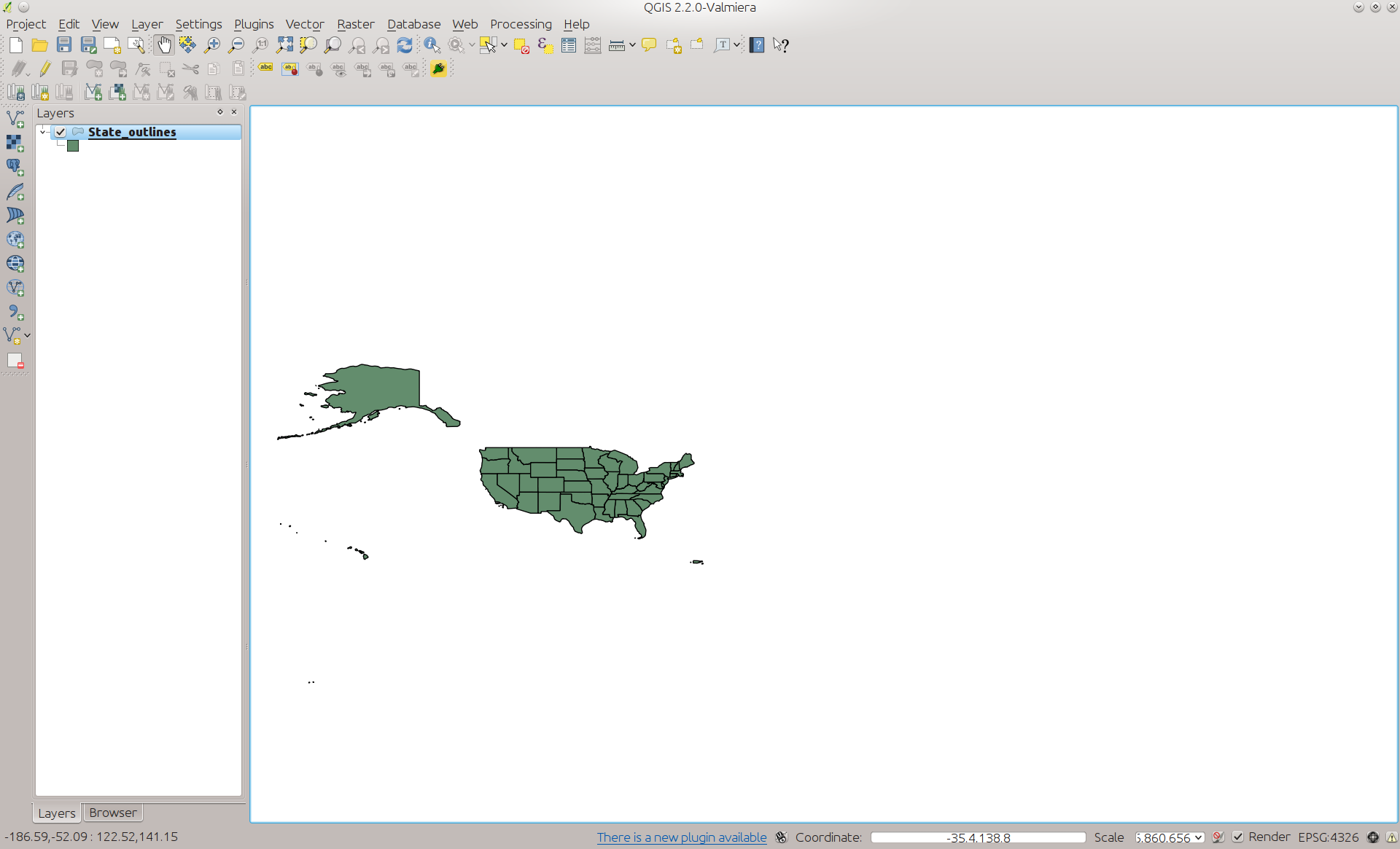
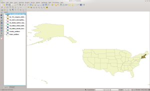
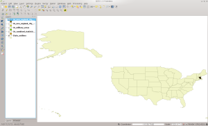
Run QGIS and load the state table that you created in the last installment. Once that finishes, add the county_outlines layer. Once loaded, it should look like this screen shot:

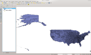
US County Outlines in QGIS

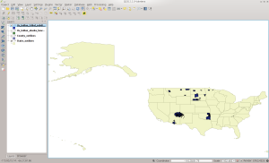
Now change to the AIANNH directory. This is the American Indian / Alaska Native / Native Hawaiian Areas dataset. This data contains information such as land and water area in each regional corporation. Run the following commands to unzip and load the data into PostGIS, substituting values specific to your setup:

[bmaddox@girls AIANNH]$ unzip tl_2013_us_aiannh.zip 
Archive: tl_2013_us_aiannh.zip
inflating: tl_2013_us_aiannh.dbf 
inflating: tl_2013_us_aiannh.prj 
inflating: tl_2013_us_aiannh.shp 
inflating: tl_2013_us_aiannh.shp.xml 
inflating: tl_2013_us_aiannh.shx 
[bmaddox@girls AIANNH]$ ls -l
total 21576
-rwxrwxr-x 1 bmaddox bmaddox 232620 Aug 6 2013 tl_2013_us_aiannh.dbf
-rwxrwxr-x 1 bmaddox bmaddox 165 Aug 6 2013 tl_2013_us_aiannh.prj
-rwxrwxr-x 1 bmaddox bmaddox 13362524 Aug 6 2013 tl_2013_us_aiannh.shp
-rwxrwxr-x 1 bmaddox bmaddox 31978 Aug 6 2013 
tl_2013_us_aiannh.shp.xml
-rwxrwxr-x 1 bmaddox bmaddox 6708 Aug 6 2013 tl_2013_us_aiannh.shx
-rwxrw-r-x 1 bmaddox bmaddox 8447076 Aug 16 2013 tl_2013_us_aiannh.zip
[bmaddox@girls AIANNH]$ shp2pgsql -s 4269 -c -D -I 
tl_2013_us_aiannh.shp US_Indian_Alaska_Hawaii_Native_Areas |psql -d 
Census_2013 
Shapefile type: Polygon
Postgis type: MULTIPOLYGON[2]
SET
SET
BEGIN
NOTICE: CREATE TABLE will create implicit sequence 
"us_indian_alaska_hawaii_native_areas_gid_seq" for serial column 
"us_indian_alaska_hawaii_native_areas.gid"
CREATE TABLE
NOTICE: ALTER TABLE / ADD PRIMARY KEY will create implicit index 
"us_indian_alaska_hawaii_native_areas_pkey" for table 
"us_indian_alaska_hawaii_native_areas"
ALTER TABLE
addgeometrycolumn 
----------------------------------------------------------------------
----------------
public.us_indian_alaska_hawaii_native_areas.geom SRID:4269 
TYPE:MULTIPOLYGON DIMS:2 
(1 row)
CREATE INDEX
COMMIT
[bmaddox@girls AIANNH]$

The loaded data should look similar to the screen shot below:

AIANNH Dataset

Next change to the AITS directory. This is the American Indian Tribal Subdivision dataset. It contains information similar to the AIANNH dataset. Since the technique should be familiar now, here are the commands to run and their output. Again, substitute the specific values applicable to your setup.

[bmaddox@girls census]$ cd AITS/
[bmaddox@girls AITS]$ ls
tl_2013_us_aitsn.zip
[bmaddox@girls AITS]$ unzip tl_2013_us_aitsn.zip 
Archive: tl_2013_us_aitsn.zip
inflating: tl_2013_us_aitsn.dbf 
inflating: tl_2013_us_aitsn.prj 
inflating: tl_2013_us_aitsn.shp 
inflating: tl_2013_us_aitsn.shp.xml 
inflating: tl_2013_us_aitsn.shx 
[bmaddox@girls AITS]$ ls -l
total 14900
-rwxrwxr-x 1 bmaddox bmaddox 134814 Aug 6 2013 tl_2013_us_aitsn.dbf
-rwxrwxr-x 1 bmaddox bmaddox 165 Aug 6 2013 tl_2013_us_aitsn.prj
-rwxrwxr-x 1 bmaddox bmaddox 9291396 Aug 6 2013 tl_2013_us_aitsn.shp
-rwxrwxr-x 1 bmaddox bmaddox 21736 Aug 6 2013 tl_2013_us_aitsn.shp.xml
-rwxrwxr-x 1 bmaddox bmaddox 3884 Aug 6 2013 tl_2013_us_aitsn.shx
-rwxrw-r-x 1 bmaddox bmaddox 5794063 Aug 16 2013 tl_2013_us_aitsn.zip
[bmaddox@girls AITS]$ shp2pgsql -s 4269 -c -D -I -WLATIN1 tl_2013_us_aitsn.shp US_Indian_Tribal_Subdivisions |psql -d Census_2013 
Shapefile type: Polygon
Postgis type: MULTIPOLYGON[2]
SET
SET
BEGIN
NOTICE: CREATE TABLE will create implicit sequence "us_indian_tribal_subdivisions_gid_seq" for serial column "us_indian_tribal_subdivisions.gid"
CREATE TABLE
NOTICE: ALTER TABLE / ADD PRIMARY KEY will create implicit index "us_indian_tribal_subdivisions_pkey" for table "us_indian_tribal_subdivisions"
ALTER TABLE
addgeometrycolumn 
-------------------------------------------------------------------------------
public.us_indian_tribal_subdivisions.geom SRID:4269 TYPE:MULTIPOLYGON DIMS:2 
(1 row)
CREATE INDEX
COMMIT
[bmaddox@girls AITS]$

The dataset should look like the following screen shot in QGIS:

AITS Dataset

Next up is the Alaska Native Regional Corporations dataset. As with the other datasets, here are the commands you will use to load the data into PostGIS:

[bmaddox@girls census]$ cd ANRC
[bmaddox@girls ANRC]$ ls -l
total 752
-rwxrw-r-x 1 bmaddox bmaddox 768407 Aug 16 2013 tl_2013_02_anrc.zip
[bmaddox@girls ANRC]$ unzip tl_2013_02_anrc.zip 
Archive: tl_2013_02_anrc.zip
inflating: tl_2013_02_anrc.dbf 
inflating: tl_2013_02_anrc.prj 
inflating: tl_2013_02_anrc.shp 
inflating: tl_2013_02_anrc.shp.xml 
inflating: tl_2013_02_anrc.shx 
[bmaddox@girls ANRC]$ ls -l
total 1896
-rwxrwxr-x 1 bmaddox bmaddox 3890 Aug 6 2013 tl_2013_02_anrc.dbf
-rwxrwxr-x 1 bmaddox bmaddox 165 Aug 6 2013 tl_2013_02_anrc.prj
-rwxrwxr-x 1 bmaddox bmaddox 1131900 Aug 6 2013 tl_2013_02_anrc.shp
-rwxrwxr-x 1 bmaddox bmaddox 21487 Aug 6 2013 tl_2013_02_anrc.shp.xml
-rwxrwxr-x 1 bmaddox bmaddox 196 Aug 6 2013 tl_2013_02_anrc.shx
-rwxrw-r-x 1 bmaddox bmaddox 768407 Aug 16 2013 tl_2013_02_anrc.zip
[bmaddox@girls ANRC]$ shp2pgsql -s 4269 -c -D -I tl_2013_02_anrc.shp US_Alaska_Native_Regional_Corporations |psql -d Census_2013 
Shapefile type: Polygon
Postgis type: MULTIPOLYGON[2]
SET
SET
BEGIN
NOTICE: CREATE TABLE will create implicit sequence "us_alaska_native_regional_corporations_gid_seq" for serial column "us_alaska_native_regional_corporations.gid"
CREATE TABLE
NOTICE: ALTER TABLE / ADD PRIMARY KEY will create implicit index "us_alaska_native_regional_corporations_pkey" for table "us_alaska_native_regional_corporations"
ALTER TABLE
addgeometrycolumn ----------------------------------------------------------------------------------------
public.us_alaska_native_regional_corporations.geom SRID:4269 TYPE:MULTIPOLYGON DIMS:2 
(1 row)

CREATE INDEX
COMMIT
[bmaddox@girls ANRC]$

Here is the screenshot of how the data should look in QGIS:

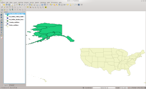
ANRC Dataset

Next change to the CBSA directory. This contains the combined Metropolitan and Micropolitan statistical areas. As before, here are the commands and you will replace things with information specific to your setup:

[bmaddox@girls census]$ cd CBSA/
[bmaddox@girls CBSA]$ ls -l
total 28960
-rwxrw-r-x 1 bmaddox bmaddox 29654427 Aug 16 2013 tl_2013_us_cbsa.zip
[bmaddox@girls CBSA]$ unzip tl_2013_us_cbsa.zip 
Archive: tl_2013_us_cbsa.zip
inflating: tl_2013_us_cbsa.dbf 
inflating: tl_2013_us_cbsa.prj 
inflating: tl_2013_us_cbsa.shp 
inflating: tl_2013_us_cbsa.shp.xml 
inflating: tl_2013_us_cbsa.shx 
[bmaddox@girls CBSA]$ ls -l
total 75708
-rwxrwxr-x 1 bmaddox bmaddox 254035 Aug 6 2013 tl_2013_us_cbsa.dbf
-rwxrwxr-x 1 bmaddox bmaddox 165 Aug 6 2013 tl_2013_us_cbsa.prj
-rwxrwxr-x 1 bmaddox bmaddox 47575788 Aug 6 2013 tl_2013_us_cbsa.shp
-rwxrwxr-x 1 bmaddox bmaddox 17767 Aug 6 2013 tl_2013_us_cbsa.shp.xml
-rwxrwxr-x 1 bmaddox bmaddox 7532 Aug 6 2013 tl_2013_us_cbsa.shx
-rwxrw-r-x 1 bmaddox bmaddox 29654427 Aug 16 2013 tl_2013_us_cbsa.zip
[bmaddox@girls CBSA]$ shp2pgsql -s 4269 -c -D -I -WLATIN1 tl_2013_us_cbsa.shp US_Metro_Micropolitan_Statistical_Areas |psql -d Census_2013 
Shapefile type: Polygon
Postgis type: MULTIPOLYGON[2]
SET
SET
BEGIN
NOTICE: CREATE TABLE will create implicit sequence "us_metro_micropolitan_statistical_areas_gid_seq" for serial column "us_metro_micropolitan_statistical_areas.gid"
CREATE TABLE
NOTICE: ALTER TABLE / ADD PRIMARY KEY will create implicit index "us_metro_micropolitan_statistical_areas_pkey" for table "us_metro_micropolitan_statistical_areas"
ALTER TABLE
addgeometrycolumn 
-----------------------------------------------------------------------------------------
public.us_metro_micropolitan_statistical_areas.geom SRID:4269 TYPE:MULTIPOLYGON DIMS:2 
(1 row)
CREATE INDEX
COMMIT
[bmaddox@girls CBSA]$

Here is how it looks in QGIS once loaded:

CBSA in QGIS

Now change to the CD directory. This dataset contains the 113^th Congress Congressional districts.

[bmaddox@girls census]$ ls CD
tl_2013_us_cd113.zip
[bmaddox@girls census]$ cd CD/
[bmaddox@girls CD]$ ls -l
total 38528
-rwxrw-r-x 1 bmaddox bmaddox 39448037 Aug 16 2013 tl_2013_us_cd113.zip
[bmaddox@girls CD]$ unzip tl_2013_us_cd113.zip 
Archive: tl_2013_us_cd113.zip
inflating: tl_2013_us_cd113.dbf 
inflating: tl_2013_us_cd113.prj 
inflating: tl_2013_us_cd113.shp 
inflating: tl_2013_us_cd113.shp.xml 
inflating: tl_2013_us_cd113.shx 
[bmaddox@girls CD]$ ls -l
total 100132
-rwxrwxr-x 1 bmaddox bmaddox 50146 Aug 6 2013 tl_2013_us_cd113.dbf
-rwxrwxr-x 1 bmaddox bmaddox 165 Aug 6 2013 tl_2013_us_cd113.prj
-rwxrwxr-x 1 bmaddox bmaddox 62997500 Aug 6 2013 tl_2013_us_cd113.shp
-rwxrwxr-x 1 bmaddox bmaddox 19400 Aug 6 2013 tl_2013_us_cd113.shp.xml
-rwxrwxr-x 1 bmaddox bmaddox 3652 Aug 6 2013 tl_2013_us_cd113.shx
-rwxrw-r-x 1 bmaddox bmaddox 39448037 Aug 16 2013 tl_2013_us_cd113.zip
[bmaddox@girls CD]$ shp2pgsql -s 4269 -c -D -I tl_2013_us_cd113.shp US_113_Congress_Districts |psql -d Census_2013 
Shapefile type: Polygon
Postgis type: MULTIPOLYGON[2]
SET
SET
BEGIN
NOTICE: CREATE TABLE will create implicit sequence "us_113_congress_districts_gid_seq" for serial column "us_113_congress_districts.gid"
CREATE TABLE
NOTICE: ALTER TABLE / ADD PRIMARY KEY will create implicit index "us_113_congress_districts_pkey" for table "us_113_congress_districts"
ALTER TABLE
addgeometrycolumn 
---------------------------------------------------------------------------
public.us_113_congress_districts.geom SRID:4269 TYPE:MULTIPOLYGON DIMS:2 
(1 row)
CREATE INDEX
COMMIT
[bmaddox@girls CD]$

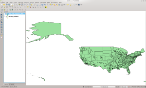
113th Congressional Districts

Now we move to the CNECTA directory.  This dataset is the Combined New England City and Town Areas dataset.

[bmaddox@girls census]$ ls CNECTA/
tl_2013_us_cnecta.zip
[bmaddox@girls census]$ cd CNECTA/
[bmaddox@girls CNECTA]$ ls -l
total 436
-rwxrw-r-x 1 bmaddox bmaddox 442433 Aug 16 2013 tl_2013_us_cnecta.zip
[bmaddox@girls CNECTA]$ unzip tl_2013_us_cnecta.zip 
Archive: tl_2013_us_cnecta.zip
inflating: tl_2013_us_cnecta.dbf 
inflating: tl_2013_us_cnecta.prj 
inflating: tl_2013_us_cnecta.shp 
inflating: tl_2013_us_cnecta.shp.xml 
inflating: tl_2013_us_cnecta.shx 
[bmaddox@girls CNECTA]$ ls -l
total 1128
-rwxrwxr-x 1 bmaddox bmaddox 1944 Aug 6 2013 tl_2013_us_cnecta.dbf
-rwxrwxr-x 1 bmaddox bmaddox 165 Aug 6 2013 tl_2013_us_cnecta.prj
-rwxrwxr-x 1 bmaddox bmaddox 679436 Aug 6 2013 tl_2013_us_cnecta.shp
-rwxrwxr-x 1 bmaddox bmaddox 16353 Aug 6 2013 tl_2013_us_cnecta.shp.xml
-rwxrwxr-x 1 bmaddox bmaddox 148 Aug 6 2013 tl_2013_us_cnecta.shx
-rwxrw-r-x 1 bmaddox bmaddox 442433 Aug 16 2013 tl_2013_us_cnecta.zip
[bmaddox@girls CNECTA]$ shp2pgsql -s 4269 -c -D -I tl_2013_us_cnecta.shp US_Combined_New_England_City_Town_Areas |psql -d Census_2013 
Shapefile type: Polygon
Postgis type: MULTIPOLYGON[2]
SET
SET
BEGIN
NOTICE: CREATE TABLE will create implicit sequence "us_combined_new_england_city_town_areas_gid_seq" for serial column "us_combined_new_england_city_town_areas.gid"
CREATE TABLE
NOTICE: ALTER TABLE / ADD PRIMARY KEY will create implicit index "us_combined_new_england_city_town_areas_pkey" for table "us_combined_new_england_city_town_areas"
ALTER TABLE
addgeometrycolumn 
-----------------------------------------------------------------------------------------
public.us_combined_new_england_city_town_areas.geom SRID:4269 TYPE:MULTIPOLYGON DIMS:2 
(1 row)
CREATE INDEX
COMMIT
[bmaddox@girls CNECTA]$

The loaded data should look similar to below:

CNECTA Dataset

Next we move on to the COAST directory. This is the US Coastline data derived from Census edges.

[bmaddox@girls census]$ ls COAST/
tl_2013_us_coastline.zip
[bmaddox@girls census]$ cd COAST/
[bmaddox@girls COAST]$ ls -l
total 15792
-rwxrw-r-x 1 bmaddox bmaddox 16168901 Aug 16 2013 tl_2013_us_coastline.zip
[bmaddox@girls COAST]$ unzip tl_2013_us_coastline.zip
Archive: tl_2013_us_coastline.zip
inflating: tl_2013_us_coastline.dbf
inflating: tl_2013_us_coastline.prj
inflating: tl_2013_us_coastline.shp
inflating: tl_2013_us_coastline.shp.xml
inflating: tl_2013_us_coastline.shx
[bmaddox@girls COAST]$ ls -l
total 40272
-rwxrwxr-x 1 bmaddox bmaddox 449644 Aug 6 2013 tl_2013_us_coastline.dbf
-rwxrwxr-x 1 bmaddox bmaddox 165 Aug 6 2013 tl_2013_us_coastline.prj
-rwxrwxr-x 1 bmaddox bmaddox 24558540 Aug 6 2013 tl_2013_us_coastline.shp
-rwxrwxr-x 1 bmaddox bmaddox 15352 Aug 7 2013 tl_2013_us_coastline.shp.xml
-rwxrwxr-x 1 bmaddox bmaddox 34028 Aug 6 2013 tl_2013_us_coastline.shx
-rwxrw-r-x 1 bmaddox bmaddox 16168901 Aug 16 2013 tl_2013_us_coastline.zip
[bmaddox@girls COAST]$ shp2pgsql -s 4269 -c -D -I -WLATIN1 tl_2013_us_coastline.shp US_Coastlines |psql -d Census_2013
Shapefile type: Arc
Postgis type: MULTILINESTRING[2]
SET
SET
BEGIN
NOTICE: CREATE TABLE will create implicit sequence "us_coastlines_gid_seq" for serial column "us_coastlines.gid"
CREATE TABLE
NOTICE: ALTER TABLE / ADD PRIMARY KEY will create implicit index "us_coastlines_pkey" for table "us_coastlines"
ALTER TABLE
addgeometrycolumn
 ------------------------------------------------------------------
public.us_coastlines.geom SRID:4269 TYPE:MULTILINESTRING DIMS:2
(1 row)
CREATE INDEX
COMMIT
[bmaddox@girls COAST]$

The coastlines will look like this:

COAST in QGIS

We now move to the CSA directory, which holds the combined statistical area national-level shapefile. These are generally areas where several large cities are combined into a single statistical unit, such as the Branson-Springfield area in Missouri.

[bmaddox@girls census]$ ls CSA
tl_2013_us_csa.zip
[bmaddox@girls census]$ cd CSA/
[bmaddox@girls CSA]$ ls -l
total 10020
-rwxrw-r-x 1 bmaddox bmaddox 10259685 Aug 16 2013 tl_2013_us_csa.zip [bmaddox@girls CSA]$ unzip tl_2013_us_csa.zip
Archive: tl_2013_us_csa.zip
inflating: tl_2013_us_csa.dbf
inflating: tl_2013_us_csa.prj
inflating: tl_2013_us_csa.shp
inflating: tl_2013_us_csa.shp.xml
inflating: tl_2013_us_csa.shx
[bmaddox@girls CSA]$ ls -l
total 26184
-rwxrwxr-x 1 bmaddox bmaddox 45139 Aug 6 2013 tl_2013_us_csa.dbf
-rwxrwxr-x 1 bmaddox bmaddox 165 Aug 6 2013 tl_2013_us_csa.prj
-rwxrwxr-x 1 bmaddox bmaddox 16477264 Aug 6 2013 tl_2013_us_csa.shp -rwxrwxr-x 1 bmaddox bmaddox 16012 Aug 6 2013 tl_2013_us_csa.shp.xml -rwxrwxr-x 1 bmaddox bmaddox 1452 Aug 6 2013 tl_2013_us_csa.shx
-rwxrw-r-x 1 bmaddox bmaddox 10259685 Aug 16 2013 tl_2013_us_csa.zip [bmaddox@girls CSA]$ shp2pgsql -s 4269 -c -D -I -WLATIN1 tl_2013_us_csa.shp US_Combined_Statistical_Areas |psql -d Census_2013
Shapefile type: Polygon
Postgis type: MULTIPOLYGON[2]
SET
SET
BEGIN
NOTICE: CREATE TABLE will create implicit sequence "us_combined_statistical_areas_gid_seq" for serial column "us_combined_statistical_areas.gid"
CREATE TABLE
NOTICE: ALTER TABLE / ADD PRIMARY KEY will create implicit index "us_combined_statistical_areas_pkey" for table "us_combined_statistical_areas"
ALTER TABLE
addgeometrycolumn
-------------------------------------------------------------------------------
public.us_combined_statistical_areas.geom SRID:4269 TYPE:MULTIPOLYGON DIMS:2
(1 row)
CREATE INDEX
COMMIT
[bmaddox@girls CSA]$

Once loaded, it should look like this in QGIS:

CSA in QGIS

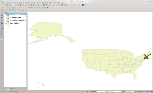
The MIL directory contains areas that are classified as belonging to the US Military… that we know about at least.

[bmaddox@girls census]$ cd MIL/
[bmaddox@girls MIL]$ dir
total 2904
-rwxrw-r-x 1 bmaddox bmaddox 2973061 Aug 16 2013 tl_2013_us_mil.zip
[bmaddox@girls MIL]$ unzip tl_2013_us_mil.zip
Archive: tl_2013_us_mil.zip
inflating: tl_2013_us_mil.dbf
inflating: tl_2013_us_mil.prj
inflating: tl_2013_us_mil.shp
inflating: tl_2013_us_mil.shp.xml
inflating: tl_2013_us_mil.shx
[bmaddox@girls MIL]$ ls -l
total 7628
-rwxrwxr-x 1 bmaddox bmaddox 150451 Aug 6 2013 tl_2013_us_mil.dbf
-rwxrwxr-x 1 bmaddox bmaddox 165 Aug 6 2013 tl_2013_us_mil.prj
-rwxrwxr-x 1 bmaddox bmaddox 4653712 Aug 6 2013 tl_2013_us_mil.shp
-rwxrwxr-x 1 bmaddox bmaddox 15575 Aug 6 2013 tl_2013_us_mil.shp.xml
-rwxrwxr-x 1 bmaddox bmaddox 6524 Aug 6 2013 tl_2013_us_mil.shx
-rwxrw-r-x 1 bmaddox bmaddox 2973061 Aug 16 2013 tl_2013_us_mil.zip
[bmaddox@girls MIL]$ shp2pgsql -s 4269 -c -D -I tl_2013_us_mil.shp US_Military_Areas |psql -d Census_2013
Shapefile type: Polygon
Postgis type: MULTIPOLYGON[2]
SET
SET
BEGIN
NOTICE: CREATE TABLE will create implicit sequence "us_military_areas_gid_seq" for serial column "us_military_areas.gid"
CREATE TABLE
NOTICE: ALTER TABLE / ADD PRIMARY KEY will create implicit index "us_military_areas_pkey" for table "us_military_areas"
ALTER TABLE
addgeometrycolumn
-------------------------------------------------------------------
public.us_military_areas.geom SRID:4269 TYPE:MULTIPOLYGON DIMS:2
(1 row)
CREATE INDEX
COMMIT
[bmaddox@girls MIL]$

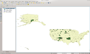
And it looks like this in QGIS:

MIL in QGIS

Now to NECTA, which is the New England City and Town Areas.

[bmaddox@girls census]$ cd NECTA
[bmaddox@girls NECTA]$ ls
tl_2013_us_necta.zip
[bmaddox@girls NECTA]$ unzip tl_2013_us_necta.zip
Archive: tl_2013_us_necta.zip
inflating: tl_2013_us_necta.dbf
inflating: tl_2013_us_necta.prj
inflating: tl_2013_us_necta.shp
inflating: tl_2013_us_necta.shp.xml
inflating: tl_2013_us_necta.shx
[bmaddox@girls NECTA]$ shp2pgsql -s 4269 -c -D -I tl_2013_us_necta.shp US_New_England_City_Town_Areas |psql -d Census_2013
Shapefile type: Polygon
Postgis type: MULTIPOLYGON[2]
SET
SET
BEGIN
NOTICE: CREATE TABLE will create implicit sequence "us_new_england_city_town_areas_gid_seq" for serial column "us_new_england_city_town_areas.gid"
CREATE TABLE
NOTICE: ALTER TABLE / ADD PRIMARY KEY will create implicit index "us_new_england_city_town_areas_pkey" for table "us_new_england_city_town_areas"
ALTER TABLE
addgeometrycolumn
--------------------------------------------------------------------------------
public.us_new_england_city_town_areas.geom SRID:4269 TYPE:MULTIPOLYGON DIMS:2
(1 row)
CREATE INDEX
COMMIT
[bmaddox@girls NECTA]$

Which looks like this in QGIS:

NECTA in QGIS

And the NECTADIV, which are the divisions in the NECTA dataset.

[bmaddox@girls census]$ cd NECTADIV/
[bmaddox@girls NECTADIV]$ dir
total 184
-rwxrw-r-x 1 bmaddox bmaddox 186486 Aug 16 2013 tl_2013_us_nectadiv.zip
[bmaddox@girls NECTADIV]$ unzip tl_2013_us_nectadiv.zip
Archive: tl_2013_us_nectadiv.zip
inflating: tl_2013_us_nectadiv.dbf
inflating: tl_2013_us_nectadiv.prj
inflating: tl_2013_us_nectadiv.shp
inflating: tl_2013_us_nectadiv.shp.xml
inflating: tl_2013_us_nectadiv.shx
[bmaddox@girls NECTADIV]$ shp2pgsql -s 4269 -c -D -I tl_2013_us_nectadiv.shp US_New_England_City_Town_Divisions |psql -d Census_2013
Shapefile type: Polygon
Postgis type: MULTIPOLYGON[2]
SET
SET
BEGIN
NOTICE: CREATE TABLE will create implicit sequence "us_new_england_city_town_divisions_gid_seq" for serial column "us_new_england_city_town_divisions.gid"
CREATE TABLE
NOTICE: ALTER TABLE / ADD PRIMARY KEY will create implicit index "us_new_england_city_town_divisions_pkey" for table "us_new_england_city_town_divisions"
ALTER TABLE
addgeometrycolumn
------------------------------------------------------------------------------------
public.us_new_england_city_town_divisions.geom SRID:4269 TYPE:MULTIPOLYGON DIMS:2
(1 row)
CREATE INDEX
COMMIT
[bmaddox@girls NECTADIV]$

QGIS Screenshot:

NECTADIV in QGIS

RAILS contains, you guessed it, the national-level file of US railroads.

[bmaddox@girls RAILS]$ dir
total 40660
-rwxrw-r-x 1 bmaddox bmaddox 41634270 Aug 16 2013 tl_2013_us_rails.zip
[bmaddox@girls RAILS]$ unzip tl_2013_us_rails.zip
Archive: tl_2013_us_rails.zip
inflating: tl_2013_us_rails.dbf
inflating: tl_2013_us_rails.prj
inflating: tl_2013_us_rails.shp
inflating: tl_2013_us_rails.shp.xml
inflating: tl_2013_us_rails.shx
[bmaddox@girls RAILS]$ ls -l
total 130320
-rwxrwxr-x 1 bmaddox bmaddox 23419778 Aug 6 2013 tl_2013_us_rails.dbf
-rwxrwxr-x 1 bmaddox bmaddox 165 Aug 6 2013 tl_2013_us_rails.prj
-rwxrwxr-x 1 bmaddox bmaddox 66902500 Aug 6 2013 tl_2013_us_rails.shp
-rwxrwxr-x 1 bmaddox bmaddox 15759 Aug 6 2013 tl_2013_us_rails.shp.xml
-rwxrwxr-x 1 bmaddox bmaddox 1463828 Aug 6 2013 tl_2013_us_rails.shx
-rwxrw-r-x 1 bmaddox bmaddox 41634270 Aug 16 2013 tl_2013_us_rails.zip
[bmaddox@girls RAILS]$ shp2pgsql -s 4269 -c -D -I tl_2013_us_rails.shp US_Rails |psql -d Census_2013
Shapefile type: Arc
Postgis type: MULTILINESTRING[2]
SET
SET
BEGIN
NOTICE: CREATE TABLE will create implicit sequence "us_rails_gid_seq" for serial column "us_rails.gid"
CREATE TABLE
NOTICE: ALTER TABLE / ADD PRIMARY KEY will create implicit index "us_rails_pkey" for table "us_rails"
ALTER TABLE
addgeometrycolumn
-------------------------------------------------------------
public.us_rails.geom SRID:4269 TYPE:MULTILINESTRING DIMS:2
(1 row)
CREATE INDEX
COMMIT
[bmaddox@girls RAILS]$

In QGIS:

RAILS in QGIS

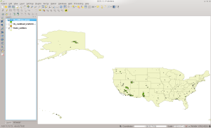
Next is TBG, which are national-level Tribal Block Groups.

[bmaddox@girls census]$ cd TBG/
[bmaddox@girls TBG]$ ls -l
total 16208
-rwxrwxr-x 1 bmaddox bmaddox 90939 Aug 6 2013 tl_2013_us_tbg.dbf
-rwxrwxr-x 1 bmaddox bmaddox 165 Aug 6 2013 tl_2013_us_tbg.prj
rwxrwxr-x 1 bmaddox bmaddox 16468896 Aug 6 2013 tl_2013_us_tbg.shp
-rwxrwxr-x 1 bmaddox bmaddox 17719 Aug 6 2013 tl_2013_us_tbg.shp.xml
-rwxrwxr-x 1 bmaddox bmaddox 7420 Aug 6 2013 tl_2013_us_tbg.shx
[bmaddox@girls TBG]$ shp2pgsql -s 4269 -c -D -I tl_2013_us_tbg.shp US_Tribal_Block_Groups |psql -d Census_2013
Shapefile type: Polygon
Postgis type: MULTIPOLYGON[2]
SET
SET
BEGIN
NOTICE: CREATE TABLE will create implicit sequence "us_tribal_block_groups_gid_seq" for serial column "us_tribal_block_groups.gid"
CREATE TABLE
NOTICE: ALTER TABLE / ADD PRIMARY KEY will create implicit index "us_tribal_block_groups_pkey" for table "us_tribal_block_groups"
ALTER TABLE
addgeometrycolumn
------------------------------------------------------------------------
public.us_tribal_block_groups.geom SRID:4269 TYPE:MULTIPOLYGON DIMS:2
(1 row)
CREATE INDEX
COMMIT
[bmaddox@girls TBG]$

In QGIS:

TBG in QGIS

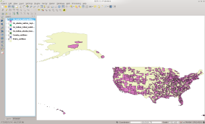
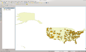
UAC contains the Urban Areas from the 2010 Census.

[bmaddox@girls census]$ cd UAC
[bmaddox@girls UAC]$ unzip tl_2013_us_uac10.zip
Archive: tl_2013_us_uac10.zip
inflating: tl_2013_us_uac10.dbf
inflating: tl_2013_us_uac10.prj
inflating: tl_2013_us_uac10.shp
inflating: tl_2013_us_uac10.shp.xml
inflating: tl_2013_us_uac10.shx
[bmaddox@girls UAC]$ ls -l
total 211884
-rwxrwxr-x 1 bmaddox bmaddox 976289 Jul 26 2013 tl_2013_us_uac10.dbf
-rwxrwxr-x 1 bmaddox bmaddox 165 Jul 26 2013 tl_2013_us_uac10.prj
-rwxrwxr-x 1 bmaddox bmaddox 132331308 Jul 26 2013 tl_2013_us_uac10.shp
-rwxrwxr-x 1 bmaddox bmaddox 17734 Aug 2 2013 tl_2013_us_uac10.shp.xml
-rwxrwxr-x 1 bmaddox bmaddox 28908 Jul 26 2013 tl_2013_us_uac10.shx
-rwxrw-r-x 1 bmaddox bmaddox 83595662 Aug 16 2013 tl_2013_us_uac10.zip
[bmaddox@girls UAC]$ shp2pgsql -s 4269 -c -D -I -WLATIN1 tl_2013_us_uac10.shp US_Urban_Areas_2010 |psql -d Census_2013
Shapefile type: Polygon
Postgis type: MULTIPOLYGON[2]
SET
SET
BEGIN
NOTICE: CREATE TABLE will create implicit sequence "us_urban_areas_2010_gid_seq" for serial column "us_urban_areas_2010.gid"
CREATE TABLE
NOTICE: ALTER TABLE / ADD PRIMARY KEY will create implicit index "us_urban_areas_2010_pkey" for table "us_urban_areas_2010"
ALTER TABLE
addgeometrycolumn
---------------------------------------------------------------------
public.us_urban_areas_2010.geom SRID:4269 TYPE:MULTIPOLYGON DIMS:2
(1 row)
CREATE INDEX
COMMIT
[bmaddox@girls UAC]$

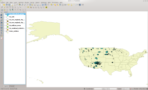
QGIS:

UAC in QGIS

Next we will do the PRIMARYROADS dataset, which can be thought of as basically major US Interstates.

[bmaddox@girls census]$ ls -l PRIMARYROADS/
total 25364
-rwxrw-r-x 1 bmaddox bmaddox 25969141 Aug 16 2013 tl_2013_us_primaryroads.zip
[bmaddox@girls census]$ cd PRIMARYROADS/
[bmaddox@girls PRIMARYROADS]$ ls -l
total 25364
-rwxrw-r-x 1 bmaddox bmaddox 25969141 Aug 16 2013 tl_2013_us_primaryroads.zip
[bmaddox@girls PRIMARYROADS]$ unzip tl_2013_us_primaryroads.zip
Archive: tl_2013_us_primaryroads.zip
inflating: tl_2013_us_primaryroads.dbf
inflating: tl_2013_us_primaryroads.prj
inflating: tl_2013_us_primaryroads.shp
inflating: tl_2013_us_primaryroads.shp.xml
inflating: tl_2013_us_primaryroads.shx
[bmaddox@girls PRIMARYROADS]$ ls -l
total 66828
-rwxrwxr-x 1 bmaddox bmaddox 1633818 Aug 6 2013 tl_2013_us_primaryroads.dbf
-rwxrwxr-x 1 bmaddox bmaddox 165 Aug 6 2013 tl_2013_us_primaryroads.prj
-rwxrwxr-x 1 bmaddox bmaddox 40696696 Aug 6 2013 tl_2013_us_primaryroads.shp
-rwxrwxr-x 1 bmaddox bmaddox 16481 Aug 6 2013 tl_2013_us_primaryroads.shp.xml
-rwxrwxr-x 1 bmaddox bmaddox 101412 Aug 6 2013 tl_2013_us_primaryroads.shx
-rwxrw-r-x 1 bmaddox bmaddox 25969141 Aug 16 2013 tl_2013_us_primaryroads.zip
[bmaddox@girls PRIMARYROADS]$ shp2pgsql -s 4269 -c -D -I -WLATIN1 tl_2013_us_primaryroads.shp US_Primary_Roads |psql -d Census_2013 Shapefile type: Arc
Postgis type: MULTILINESTRING[2]
SET
SET
BEGIN
NOTICE: CREATE TABLE will create implicit sequence "us_primary_roads_gid_seq" for serial column "us_primary_roads.gid" CREATE TABLE
NOTICE: ALTER TABLE / ADD PRIMARY KEY will create implicit index "us_primary_roads_pkey" for table "us_primary_roads"
ALTER TABLE
addgeometrycolumn
---------------------------------------------------------------------
public.us_primary_roads.geom SRID:4269 TYPE:MULTILINESTRING DIMS:2 (1 row)
CREATE INDEX
COMMIT
[bmaddox@girls PRIMARYROADS]$

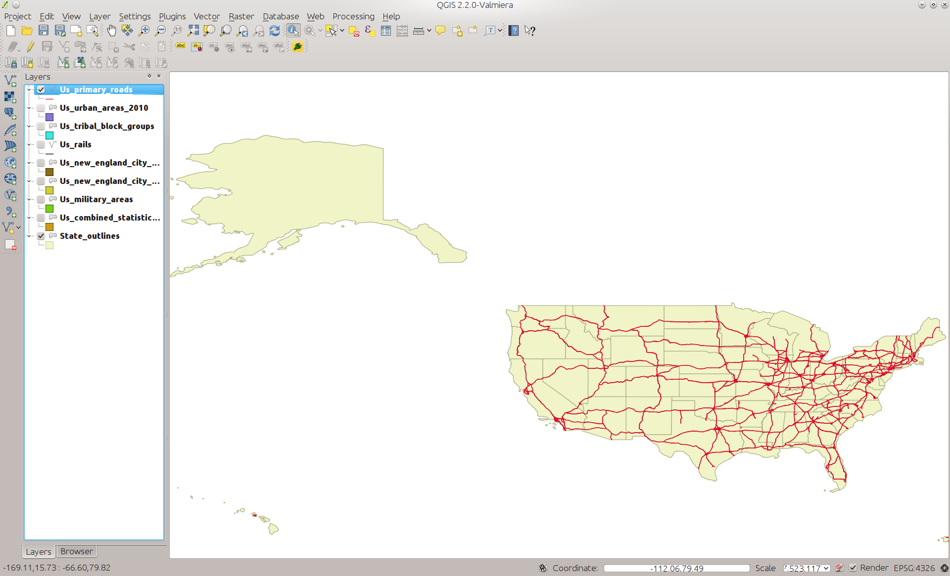
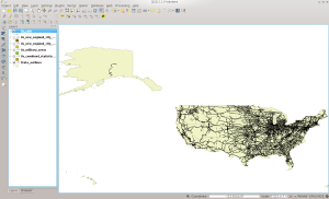
And in QGIS:

PRIMARYROADS in QGIS

And finally (yes FINALLY!), the ZCTA5 dataset, which is the list of US zip code tabulation areas.

[bmaddox@girls census]$ cd ZCTA5/
[bmaddox@girls ZCTA5]$ dir
total 513180
-rwxrw-r-x 1 bmaddox bmaddox 525492077 Aug 16 2013 tl_2013_us_zcta510.zip
[bmaddox@girls ZCTA5]$ unzip tl_2013_us_zcta510.zip
Archive: tl_2013_us_zcta510.zip
inflating: tl_2013_us_zcta510.dbf
inflating: tl_2013_us_zcta510.prj
inflating: tl_2013_us_zcta510.shp
inflating: tl_2013_us_zcta510.shp.xml
inflating: tl_2013_us_zcta510.shx
[bmaddox@girls ZCTA5]$ shp2pgsql -s 4269 -c -D -I -WLATIN1 tl_2013_us_zcta510.shp US_Zip_Code_Areas |psql -d Census_2013
Shapefile type: Polygon
Postgis type: MULTIPOLYGON[2]
SET
SET
BEGIN
NOTICE: CREATE TABLE will create implicit sequence "us_zip_code_areas_gid_seq" for serial column "us_zip_code_areas.gid"
CREATE TABLE
NOTICE: ALTER TABLE / ADD PRIMARY KEY will create implicit index "us_zip_code_areas_pkey" for table "us_zip_code_areas"
ALTER TABLE
addgeometrycolumn
------------------------------------------------------------------- public.us_zip_code_areas.geom SRID:4269 TYPE:MULTIPOLYGON DIMS:2
(1 row)
CREATE INDEX
COMMIT
[bmaddox@girls ZCTA5]$

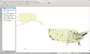
And the final screen shot:

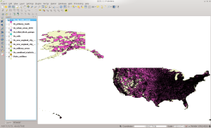
ZCTA5 in QGIS

So that is it. You now have the US state borders, county outlines, and a large amount of national-level data such as railroads and interstates. In 8.3 we will tackle some of the other datasets that are comprised of multiple county files for each state. We will convert them to single state files and then import them into PostGIS. Until then, examine and experiment with what you have just done and see what data is actually inside the tables.

In this installment we focus on downloading, condensing, and uploading US Census TIGER data into PostGIS. The complete TIGER dataset is very large, and you should allocate enough time and space to download it all. As we go along, I will let you know how big a download you can expect and how much temporary space you will need to process them. I will be describing how to download, convert, and upload the files using my Ubuntu system. The instructions will be a bit different using Windows and you should consult your documentation as to how the utilities run there. I will be using the lftp program to download the files, tools from GDAL to do the processing, and shp2pgsql from PostGIS to upload the data.

The Census portion of the series covers a lot of information, so I am breaking it up into multiple parts to avoid having you fall asleep while reading a large document. This part focuses on the layout of the Census FTP site and what files are contained in each directory. I am also including pointers to the full Census TIGER documentation for a reading assignment. At the end, I will go over importing the Census state outlines so you at least have something to look at until next time.

I will be posting my own conversions of the TIGER dataset to this website. The Census puts data out at a county level. Personally, I prefer having the data at a state level and that is also how I import it into PostGIS. Plus, having it backed up at the state level is handy in case you accidentally blow away your data like I may have done just recently while preparing for this part of the series. So if you like, you could read along and then just download the condensed file from my site if you do not feel like running the conversions on your own.

At the time of this writing, the latest version of the data is 2013 and is available at http://www.census.gov/geo/maps-data/data/tiger-line.html. The Census makes the data available for download in Shapefile format inside of zip files for each county or national organizational unit. The first thing you should do is skim through the full technical documentation that is available in PDF format here. This document describes the data model used in the various file sets and what each field means inside the various files. It also describes what the files contain and their naming convention. This information is very useful if you intend to do more than just load data to look at a map.

We will be downloading the data from the main FTP site here. I will be using the lftp program under Linux to download the files, as it provides an easy way to download entire directories at a time. On Windows there are similar download managers you can use to accomplish the same task. When you ftp to the above site, you will see the following directory structure:

lftp ftp2.census.gov:/geo/tiger/TIGER2013> dir
-rw-rw-r-- 1 holla301 i-geo 228662 Aug 21 2013 2013-FolderNames-Defined.pdf
drwxrwsr-x 2 holla301 i-geo 143360 Aug 16 2013 ADDR
drwxrwsr-x 2 holla301 i-geo 167936 Aug 16 2013 ADDRFEAT
drwxrwsr-x 2 holla301 i-geo 143360 Aug 16 2013 ADDRFN
drwxrwsr-x 2 holla301 i-geo 4096 Aug 16 2013 AIANNH
drwxrwsr-x 2 holla301 i-geo 4096 Aug 16 2013 AITS
drwxrwsr-x 2 holla301 i-geo 4096 Aug 16 2013 ANRC
drwxrwsr-x 2 holla301 i-geo 4096 Aug 16 2013 AREALM
drwxrwsr-x 2 holla301 i-geo 167936 Aug 16 2013 AREAWATER
drwxrwsr-x 2 holla301 i-geo 4096 Aug 16 2013 BG
drwxrwsr-x 2 holla301 i-geo 4096 Aug 16 2013 CBSA
drwxrwsr-x 2 holla301 i-geo 4096 Aug 16 2013 CD
drwxrwsr-x 2 holla301 i-geo 4096 Aug 16 2013 CNECTA
drwxrwsr-x 2 holla301 i-geo 4096 Aug 16 2013 COAST
drwxrwsr-x 2 holla301 i-geo 4096 Aug 16 2013 CONCITY
drwxrwsr-x 2 holla301 i-geo 4096 Aug 16 2013 COUNTY
drwxrwsr-x 2 holla301 i-geo 4096 Aug 16 2013 COUSUB
drwxrwsr-x 2 holla301 i-geo 4096 Aug 16 2013 CSA
drwxrwsr-x 2 holla301 i-geo 135168 Aug 16 2013 EDGES
drwxrwsr-x 2 holla301 i-geo 4096 Aug 16 2013 ELSD
drwxrwsr-x 2 holla301 i-geo 4096 Aug 16 2013 ESTATE
drwxrwsr-x 2 holla301 i-geo 147456 Sep 13 12:24 FACES
drwxrwsr-x 2 holla301 i-geo 172032 Aug 16 2013 FACESAH
drwxrwsr-x 2 holla301 i-geo 4096 Aug 16 2013 FACESAL
drwxrwsr-x 2 holla301 i-geo 4096 Aug 16 2013 FACESMIL
drwxrwsr-x 2 holla301 i-geo 163840 Aug 16 2013 FEATNAMES
drwxrwsr-x 2 holla301 i-geo 180224 Aug 16 2013 LINEARWATER
drwxrwsr-x 2 holla301 i-geo 4096 Aug 16 2013 METDIV
drwxrwsr-x 2 holla301 i-geo 4096 Aug 16 2013 MIL
drwxrwsr-x 2 holla301 i-geo 4096 Aug 16 2013 NECTA
drwxrwsr-x 2 holla301 i-geo 4096 Aug 16 2013 NECTADIV
drwxrwsr-x 2 holla301 i-geo 126976 Aug 16 2013 OTHERID
drwxrwsr-x 2 holla301 i-geo 4096 Aug 16 2013 PLACE
drwxrwsr-x 2 holla301 i-geo 4096 Aug 16 2013 POINTLM
drwxrwsr-x 2 holla301 i-geo 4096 Aug 16 2013 PRIMARYROADS
drwxrwsr-x 2 holla301 i-geo 4096 Aug 16 2013 PRISECROADS
drwxrwsr-x 2 holla301 i-geo 4096 Aug 16 2013 PUMA
drwxrwsr-x 2 holla301 i-geo 4096 Aug 16 2013 RAILS
drwxrwsr-x 2 holla301 i-geo 155648 Aug 16 2013 ROADS
drwxrwsr-x 2 holla301 i-geo 4096 Aug 16 2013 SCSD
drwxrwsr-x 2 holla301 i-geo 4096 Aug 16 2013 SLDL
drwxrwsr-x 2 holla301 i-geo 4096 Aug 16 2013 SLDU
drwxrwsr-x 2 holla301 i-geo 4096 Aug 16 2013 STATE
drwxrwsr-x 2 holla301 i-geo 4096 Aug 16 2013 SUBMCD
drwxrwsr-x 2 holla301 i-geo 4096 Aug 16 2013 TABBLOCK
drwxrwsr-x 2 holla301 i-geo 4096 Aug 16 2013 TBG
drwxrwsr-x 2 holla301 i-geo 4096 Aug 16 2013 TRACT
drwxrwsr-x 2 holla301 i-geo 4096 Aug 16 2013 TTRACT
drwxrwsr-x 2 holla301 i-geo 4096 Aug 16 2013 UAC
drwxrwsr-x 2 holla301 i-geo 4096 Aug 16 2013 UNSD
drwxrwsr-x 2 holla301 i-geo 4096 Aug 16 2013 ZCTA5

As to what these directories contain, here is a summary taken from the TIGER documentation. As we load each file type, I will cover what the files contain in more detail.

• ADDR – Address Range Relationship File. These files contain DBF files that contain address information for each edge in the dataset. For each edge, it lists the from- and to- house numbers, which side of the road they are on, the ZIP, and ZIP+4 codes.
• ADDRFEAT – Address Range Feature File. These files are Shapefiles that contain information similar to the above and other metadata such as street names.
• ADDRFN – Address Range-Feature Name Relationship File. Each file maps the relationship between address range and linear feature identifiers.
• AIANNH – American Indian / Alaska Native / Native Hawaiian Areas. This national-level file contains federally-recognized American Indian reservations and off-reservation trust land areas, state-recognized reservations, and Hawaiian home land areas for which the Census publishes data.
• AITSN – American Indian Tribal Subdivision National. Another national-level file that contains legally defined administrative subdivisions of federally-recognized American Indian reservations, off-reservation trust lands, or Oklahoma tribal statistical areas.
• ANRC – Alaska Native Regional Corporation. These are areas that define corporate entities established to conduct both business and nonprofit affairs of the Alaska Natives pursuant to the Alaska Native Claims Settlement Act of 1972.
• AREALM – Area Landmarks. These files contain area landmarks that the Census records for locating special features and to help enumerators during field operations (parks, schools, etc).
• AREAWATER – Area Water. These contain polygonal area definitions of water (or hydrographic) features such as lakes, ponds, and rivers.
• BG – Block Groups. These are Census-specific clusters of blocks that have the same first digit of their four-digit identifying numbers within a Census Tract.
• CBSA – Metropolitan Statistical Area / Micropolitan Statistical Area. These Shapefiles contain the 2013 county and equivalent entities and contain fields with codes for combined, metropolitan, or micropolitan statistical areas and metropolitan divisions.
• CD – Congressional District. These are area definitions of the 113^th Congressional Districts.
• CNECTA – Combined New England City and Town Area. These files contain the Office of Management and Budget (OMB)-defined alternative county subdivision-based definitions of statistical areas known as New England city and town areas.
• COASTLINE – US Coastlines. This is a new addition that is a national-level file of linear coastline features.
• CONCITY – Consolidated Cities. These are defined as units of local governments for which the functions of the incorporated place and its county or minor civil division have merged.
• COUNTY – US Counties. This is a national-level file containing the definitions for counties within the US and its territories.
• COUSUB – County Subdivision. These are statistical subdivisions of boroughs, city nad boroughs, municipalities, and census areas.
• CSA – Combined Statistical Area. These are groups of two or more areas that have significant employment interchanges.
• EDGES – All linear edges in the dataset. These data contain every edge that the Census has recorded, be it road, rail, or water features.
• ELSD – Elementary School District. These are area definitions that define locality-recognized elementary school districts.
• ESTATE – Estates. These are subdivisions of the three major islands in the United States Virgin Islands that have legally defined boundaries and are generally smaller in area than the Census subdistricts.
• FACES – Topological Faces (Polygons With All Geocodes). Faces are areal objects that are bounded by one or more edges and are topological primitives. A face is not internally subdivided by edges into smaller polygons but may completely surround other faces (such as islands).
• FACESAH – Topological Faces-Area Hydrography Relationship File. These are face areas that contain a water feature relationship.
• FACESAL – Topological Faces-Area Landmark Relationship File. These are face areas that contain a landmark feature relationship.
• FACESMIL – Topological Faces-Military Installation Relationship File. These are face areas that contain a military feature relationship.
• FEATNAMES – Feature Names Relationship File. These files contain a record for each feature name-edge combination and includes the feature name attributes. This file may contain alternative names for linear features.
• LINEARWATER – Linear Water. This file contains linear features where the edge represents a water feature.
• METDIV – Metropolitan Division. These files represent metropolitan statistical areas containing a single core with a population of at least 2.5 million people and is subdivided to form smaller groupings of counties or equivalent entities.
• MIL – Military Installations. This is a national-level file denoting US military installations.
• NECTA – New England City and Town Area. These files contain the areas covered by the OMB for Combined New England city and town areas.
• NECTADIV – New England City and Town Area Division. These areas are created when a NECTA containing a single core with a population of at least 2.5 million is to form smaller groupings of cities and towns.
• OTHERID – Other Identifiers. This file contains external identifier codes and individual county identifiers between the permanent edge identifier attribute in the EDGES file and the identifier listed here.
• PLACE – Places. These files contain geography and attributes at the state level of both incorporated places and census designated places.
• POINTLM – Point Landmarks. These are point features that are used to locate special features and to help enumerators during field operations. They contain points that identify areas such as airports, parks, and schools.
• PRIMARYROADS – Primary Roads. These are defined as generally divided, limited-access highways within the Federal interstate highway system or under state management.
• PRISECROADS – Primary and Secondary Roads. These files contain the primary roads and main arteries that are usually in a US, state, or county highway system with one or more lanes of traffic in each direction.
• PUMA – Public Use Microdata Area. These are decennial census areas that have been definied for the tabulation and dissemination of public use microdata sample American Community Survey data.
• RAILS – Railroads. These are linear edges that denote railroads at the national level.
• ROADS – All roads. These files contain all roads (major or minor) in the US and its territories.
• SCSD – Secondary School District. These are secondary school districts that are typically defined as between elementary school and college.
• SLDL – State Legislative District – Lower Chamber. These areas denote state legislative districts that are equivalent to a house chamber.
• SLDU – State Legislative District – Upper Chamber. These areas denote state legislative districts that are equivalent to a senate chamber.
• STATE – State and Equivalent. These files contain the outlines of each state and territory in the US.
• SUBBARRIO – SubMinor Civil Division (Subbarrios in Puerto Rico). These areas are legally defined divisions or minor civil divisions in Puerto Rico.
• TABBLOCK – Tabulation (Census) Block. These areas are definied by the Census as statistical areas bounded on all sides by visible features, such as streets, roads, streams, railroad tracks, and by non-visible boundaries such as city, town, township, and county limits.
• TBG – Tribal Block Group. These areas are clusters of blocks within the same tribal census tract.
• TRACT – Census Tract. These areas are small, relatively permanent statistical subdivisions of a county or equivalent entity and are reviewed and updated by local participants prior to each decennial census as part of the Census Bureau’s Participant Statistical Areas Program.
• TTRACT – Tribal Census Tract. These are relatively small statistical subdivisions of an American Indian reservation and/or off-reservation trust land and were defined by federally recognized tribal government officials working with the Census.
• UAC – Urban Area/Urban Cluster. These are clusters consisting of densely developed territory that has between 2,500 and 50,000 people.
• UNSD – Unified School District. These are pseudo-secondary school districts that represent regular unified school districts in areas where the unified school district share final responsibility with the elementary district.
• ZCTA5 – 5-Digit ZIP Code Tabulation Area. These are approximate area representations of US Postal Service five digit ZIP code service areas that the Census creates using whole blocks to present statistical data from censuses and surveys.

Census State Outlines

We first need a database to hold all of the Census data. If you created a geospatial database template from earlier in this series, open a shell prompt and type:

createdb -T gistemplate Census_2013

Now that we have gone through all of that, the first dataset we will upload is only 8.3 megabytes in size. From the shell prompt, run:

mkdir census
cd census

Again from the shell prompt, run

lftp ftp://ftp2.census.gov/geo/tiger/TIGER2013.

You should see something similar to the below:

lftp ftp://ftp2.census.gov/geo/tiger/TIGER2013
cd ok, cwd=/geo/tiger/TIGER2013
lftp ftp2.census.gov:/geo/tiger/TIGER2013>

You can then type cls to get a shortened listing of the directories I just described. From inside the client, type:

mirror STATE/

lftp will download the file and once done you will see something like this:

lftp ftp2.census.gov:/geo/tiger/TIGER2013> mirror STATE/
Total: 1 directory, 1 file, 0 symlinks
New: 1 file, 0 symlinks
8599274 bytes transferred in 17 seconds (500.2K/s)
lftp ftp2.census.gov:/geo/tiger/TIGER2013>

You can now type quit and hit enter or type Control-D to exit lftp. Change into the directory STATE and you will see this file:

[bmaddox@girls STATE]$ ls -l
total 8400
-rwxrw-r-x 1 bmaddox bmaddox 8599274 Aug 16 2013 tl_2013_us_state.zip
[bmaddox@girls STATE]$

This follows the Census naming convention of:

• tl = TIGER/Line
• 2013 = the version of the files
• us = parent geography entity ID code of the geographic extent, in this case US being the entire country.
• State = layer tag for the dataset
• zip = the file extension

Run unzip tl_2013_us_state.zip and you will then find these files in the STATE directory:

[bmaddox@girls STATE]$ unzip tl_2013_us_state.zip
Archive: tl_2013_us_state.zip
inflating: tl_2013_us_state.dbf
inflating: tl_2013_us_state.prj
inflating: tl_2013_us_state.shp
inflating: tl_2013_us_state.shp.xml
inflating: tl_2013_us_state.shx
[bmaddox@girls STATE]$ ls
tl_2013_us_state.dbf tl_2013_us_state.shp tl_2013_us_state.shx
tl_2013_us_state.prj tl_2013_us_state.shp.xml tl_2013_us_state.zip
[bmaddox@girls STATE]

These files make up the ESRI Shapefile format. For a more complete explanation of what each file is, consult the links to the format that I have posted previously in this series.

To upload the files to PostGIS with the proper geographic coordinates, we need to know the EPSG code of the data that defines its projection. All Census TIGER data uses the EPSG code 4269 which denotes the NAD83 datum.

From this directory, run the following command to create a table with the state outlines and your output should look similar to the below:

[bmaddox@girls STATE]$ shp2pgsql -s 4269 -c -D -I tl_2013_us_state.shp State_Outlines | psql -d Census_2013
Shapefile type: Polygon
Postgis type: MULTIPOLYGON[2]
SET
SET
BEGIN
NOTICE: CREATE TABLE will create implicit sequence "state_outlines_gid_seq" for serial column "state_outlines.gid"
CREATE TABLE
NOTICE: ALTER TABLE / ADD PRIMARY KEY will create implicit index "state_outlines_pkey" for table "state_outlines"
ALTER TABLE
addgeometrycolumn
----------------------------------------------------------------
public.state_outlines.geom SRID:4269 TYPE:MULTIPOLYGON DIMS:2
(1 row)

CREATE INDEX
COMMIT
[bmaddox@girls STATE]$

The options to the command line are:

• -s = specify the EPSG code
• -c = create a table
• -D = use postgresql dump format (speeds things up basically)
• -I = create a spatial index column. This column contains the coordinates of the line segments so a GIS can determine where they are
• State_Outlines = the table name to create
• | psql -d Census_2013 = takes the output from the shp2pgsql command and pipes it to the psql command using the Census_2013 database.

To view the data, run QGIS Desktop. As I discussed earlier in the series, open the load from PostGIS dialog and create an entry called Census_2013 with the hostname, database, user, and password for your specific setup. Once that is done, click Connect and expand the entries under the public schema and you should see something like this:

Census 2013 Table with State Outlines

Click the state_outlines layer and then the Add button. After a second or two you should see this:

State Outlines table in QGIS

And that is it. Fairly easy, eh? You have just successfully learned a bit about the Census TIGER dataset, put data into PostGIS, and viewed it inside QGIS. You can right click on the layer in QGIS to view the attribute table to see what kind of data is stored for each state.

Next time, we will continue working through TIGER data to create your first large-scale geospatial database.