Stupid LIDAR Tricks Finale

I thought I’d finally wrap this up so I can move on to other things.  Since I’ve last posted, I replaced my Jankinator 1000 (nVidia Tesla P40 with a water cooler) and my nVidia RTX 2060 with an Intel Arc A770.  It has 16Gb of VRAM and is actually a pretty fast GPU on my Linux box.

So far I’ve had pretty good luck getting things like TensorFlow and PyTorch working on it, as mentioned in a previous blog post.  The only thing so far that I haven’t gotten to work 100% is Facebook’s Segment Anything Model 2 (SAM2) (which of course is what I mentioned in the last post I wanted to try to use with the LIDAR GeoTIFF).  Basically now down to running out of VRAM although I’m not sure exactly why since I’ve tweaked settings for OpenCL memory allocation on Linux, etc.  I’ve finally given up on that one for now and decided to just use the CPU for processing.

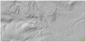
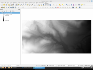
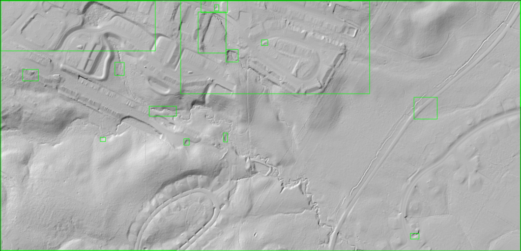
As a refresher, here is the LIDAR GeoTIFF I have been using.


SAM2 has the ability to automatically generate masks on input images.  This was of interest to me since I wanted to test it to try to automatically identify areas of interest from LIDAR.  Fortunately, the GitHub repo for SAM2 has a Jupyter notebook that made it easy to run some experiments.


With all of the default parameters, we can see that it only identified the lower right corner of the image.  I tweaked a few of the settings and came up with this version:


The second image does show some areas highlighted.  It got a grouping of row houses on the bottom of the image.  It also found a few single family houses as well.  However, it also flagged areas where there is really nothing of interest.

Finale

What have we learned from all of this?  Well, LIDAR is hard.  Automatically finding features of interest in LIDAR is also hard.  We can get some decent results using image processing and/or deep learning techniques, but as with anything in the field, we are no where near 100%.

Previously I posted about training a custom RCNN to identify features of interest from GeoTIFF LIDAR.  It was somewhat successful, although, as I said, it needed a lot more training data than I had available.

I do think that over time, people will develop models that do a good job of finding certain areas of interest in LIDAR.  Some fields already have software to find specific features in LIDAR, especially in fields such as archaeology.  And this is probably how things will continue for a while.  We probably will not have a generalized “find everything of interest in this LIDAR image” model or software for a long time.  However, it is possible to train a model to identify specific areas.

I am also working with LIDAR point data as well versus GeoTIFF versions.  Point data is a lot different beast in that it has various classifications of the points after it has been processed.  You can then do things such as extract tree canopy points or bare ground points.  Conversion to a raster necessarily looses information as things have to be interpolated and reduced in order to produce a raster.  I’ll post some things here in the future as while point cloud data can be harder to work with, I think the results are better than what can be obtained via rasters.

Posted in GIS

Saying Goodbye to my Census Tiger Data

For a long time now I’ve maintained a version of the Public Domain Census Tiger Data converted from county-level to state-level.  Over the years I’ve actually had a lot of those shape files downloaded so I’m glad they were useful to some people!

However, the Census is now putting out geopackages of there data at both the national and state levels.  I’d also like to thank the US Census for doing that as I think state-level data is way more usable than county level!

As a result, I think there’s not really a reason for me to host the state-level data any more.  I’ll still host the script to download and create a PostgreSQL/PostGIS database at my github repo, and might even get around to adding scripts to automatically process the geopackages.

So, so long my state-level Census data and thanks for all the fish!

How I Got TensorFlow and PyTorch working on an Intel Arc A770 GPU

Recently I replaced my Jankinator 1000 with an Intel Arc A770 16GB card.  While this card is a 16GB card versus 24GB, it’s a lot faster and, well, it is not an NVIDIA card. Plus, I can do things like mixed precision processing and modify batch sizes to cope with the loss of 8GB.  I will spare you my thoughts on certain companies and their monopolies in Deep Learning systems.

I thought I would write up this post since, well, some Intel documentation is a bit scattered and is not the easiest to follow. Plus some of it will end up messing with your system if you are not careful. For reference, I’m running Linux Mint 22, which is based on Ubuntu 24.04 Noble.

So for the standard disclaimer, these instructions got everything working for me.  I make absolutely no guarantees that they will work for you.  If your house burns down or a portal opens and Cthulhu appears, don’t blame me.

Drivers

First off, make sure you are running kernel version 6.8.0-41 or later. In some earlier kernels, someone posted a patch that caused a regression in the compute engines on the Arc GPUs (https://github.com/intel/compute-runtime/issues/726). This has been fixed in more recent kernels on Ubuntu. If you are on Linux Mint like I am (and would highly recommend), you should have the latest HWE kernel. If not, go ahead and install it first.

Next we will follow some of these instructions comes from Intel’s documentation at https://github.com/intel/intel-extension-for-tensorflow/blob/main/docs/install/experimental/install_for_arc_gpu.md. Note that it does not currently mention Ubuntu 24.04, but trust me, it works. We will mostly follow their documentation to properly install the drivers, just with a few changes.

Core Drivers

First set up the gpg key for the Intel repo.

sudo apt-get install -y gpg-agent wget
wget -qO - https://repositories.intel.com/gpu/intel-graphics.key | sudo gpg --dearmor --output /usr/share/keyrings/intel-graphics.gpg

Now we install the Intel GPU repository. We differ from their instructions here because while the Nobel repository is not mentioned, trust me it is there.

echo "deb [arch=amd64 signed-by=/usr/share/keyrings/intel-graphics.gpg] https://repositories.intel.com/gpu/ubuntu noble unified" | sudo tee /etc/apt/sources.list.d/intel-gpu-noble.list
sudo apt-get update

Next you will need to install the proper packages.

apt install intel-opencl-icd libze1 intel-level-zero-gpu-raytracing intel-media-va-driver-non-free libmfx1 libmfxgen1 libvpl2 libegl-mesa0 libegl1 libegl1-mesa-dev libgbm1 libgl1-mesa-dev libgl1-mesa-dri libglapi-mesa libgles2-mesa-dev libglx-mesa0 libigdgmm12 libxatracker2 mesa-va-drivers mesa-vdpau-drivers mesa-vulkan-drivers va-driver-all vainfo hwinfo clinfo

This is another difference from the Intel documentation. libze1 has replaced intel-level-zero-gpu, although intel-level-zero-gpu-raytracing is still around. Also libegl1-mesa seems to have been renamed to libegl1 except for the dev package.

You should probably reboot now since the intel-media-va-driver-non-free driver contains some extra functionality that the fully open source version does not.

One API

Now we go ahead and follow their instructions for setting up the Intel One API repository.

wget -O- https://apt.repos.intel.com/intel-gpg-keys/GPG-PUB-KEY-INTEL-SW-PRODUCTS.PUB | sudo gpg --dearmor --output /usr/share/keyrings/oneapi-archive-keyring.gpg
echo "deb [signed-by=/usr/share/keyrings/oneapi-archive-keyring.gpg] https://apt.repos.intel.com/oneapi all main" | sudo tee /etc/apt/sources.list.d/oneAPI.list
sudo apt-get update

Here we also stray a bit from their documentation. I have found we need to install a LOT of packages from One API to make sure everything works, including their TensorFlow and PyTorch extensions.

apt install intel-oneapi-runtime-dpcpp-cpp intel-oneapi-runtime-mkl intel-oneapi-common-oneapi-vars-2024.2 intel-oneapi-common-licensing-2024.2 intel-oneapi-common-vars intel-oneapi-dpcpp-ct-2024.2 intel-oneapi-mkl-cluster-2024.2 intel-oneapi-tbb-common-devel-2021.13 intel-oneapi-compiler-shared-2024.2 intel-oneapi-dal-2024.6 intel-oneapi-mkl-sycl-include-2024.2 intel-oneapi-mkl-sycl-2024.2 intel-oneapi-ippcp-common-devel-2021.12 intel-basekit-getting-started-2024.2 intel-oneapi-tlt-2024.2 intel-oneapi-advisor intel-oneapi-icc-eclipse-plugin-cpp-2024.2 intel-oneapi-openmp-common-2024.2 intel-oneapi-compiler-dpcpp-cpp-runtime-2024.2 intel-oneapi-mkl-sycl-vm-2024.2 intel-oneapi-mkl-devel-2024.2 intel-oneapi-mkl-sycl-devel-common-2024.2 intel-oneapi-ippcp-common-2021.12 intel-oneapi-dal-common-2024.6 intel-oneapi-mpi-devel-2021.13 intel-oneapi-ipp-2021.12 intel-oneapi-openmp-2024.2 intel-oneapi-dev-utilities-eclipse-cfg-2024.2 intel-oneapi-ipp-common-2021.12 intel-oneapi-tbb-2021.13 intel-oneapi-mkl-cluster-devel-common-2024.2 intel-oneapi-ipp-devel-2021.12 intel-oneapi-compiler-shared-runtime-2024.2 intel-oneapi-compiler-dpcpp-eclipse-cfg-2024.2 intel-oneapi-mkl-sycl-devel-2024.2 intel-oneapi-mkl-classic-include-2024.2 intel-oneapi-vtune intel-oneapi-mkl-core-2024.2 intel-oneapi-mkl-cluster-devel-2024.2 intel-oneapi-mkl-sycl-stats-2024.2 intel-oneapi-compiler-shared-common-2024.2 intel-oneapi-diagnostics-utility-2024.2 intel-oneapi-mkl-sycl-sparse-2024.2 intel-basekit-env-2024.2 intel-oneapi-libdpstd-devel-2022.6 intel-oneapi-mkl-sycl-blas-2024.2 intel-oneapi-dev-utilities-2024.2 intel-oneapi-dal-devel-2024.6 intel-oneapi-tbb-common-2021.13 intel-oneapi-dnnl-2024.2 intel-oneapi-mpi-2021.13 intel-oneapi-compiler-dpcpp-cpp-2024.2 intel-oneapi-mkl-classic-devel-2024.2 intel-oneapi-mkl-core-common-2024.2 intel-oneapi-ipp-common-devel-2021.12 libssl-dev intel-oneapi-mkl-core-devel-2024.2 intel-oneapi-mkl-sycl-lapack-2024.2 intel-oneapi-mkl-core-devel-common-2024.2 intel-oneapi-compiler-dpcpp-cpp-common-2024.2 intel-oneapi-mkl-sycl-data-fitting-2024.2 intel-oneapi-tbb-devel-2021.13 intel-oneapi-dpcpp-cpp-2024.2 intel-oneapi-dal-common-devel-2024.6 intel-oneapi-tcm-1.1 intel-oneapi-dpcpp-ct-eclipse-cfg-2024.2 intel-oneapi-ccl-devel-2021.13 intel-oneapi-dnnl intel-oneapi-compiler-cpp-eclipse-cfg-2024.2 intel-oneapi-mkl-sycl-rng-2024.2 intel-oneapi-mkl-classic-include-common-2024.2 intel-oneapi-ippcp-2021.12 intel-oneapi-dnnl-devel-2024.2 intel-oneapi-ccl-2021.13 intel-oneapi-mkl-sycl-dft-2024.2 intel-oneapi-dpcpp-debugger-2024.2 intel-oneapi-ippcp-devel-2021.12 intel-basekit-2024.2

Yes that is a lot of packages, but you will need them eventually.

Now add these statements in your .bashrc to ensure that all the necessary environment variables are set:

# Intel stuff
source /opt/intel/oneapi/setvars.sh
source /opt/intel/oneapi/compiler/latest/env/vars.sh
source /opt/intel/oneapi/mkl/latest/env/vars.sh

Save your .bashrc file and now whenever you open a terminal you should see something like this:

:: initializing oneAPI environment ...
bash: BASH_VERSION = 5.2.21(1)-release
args: Using "$@" for setvars.sh arguments:
:: advisor -- latest
:: ccl -- latest
:: compiler -- latest
:: dal -- latest
:: debugger -- latest
:: dev-utilities -- latest
:: dnnl -- latest
:: dpcpp-ct -- latest
:: dpl -- latest
:: ipp -- latest
:: ippcp -- latest
:: mkl -- latest
:: mpi -- latest
:: tbb -- latest
:: vtune -- latest
:: oneAPI environment initialized ::

If you want, you can run clinfo to make sure OpenCL is working on the Arc.

bmaddox@sdf1:~$ clinfo
Number of platforms 2
Platform Name Intel(R) OpenCL
Platform Vendor Intel(R) Corporation
Platform Version OpenCL 3.0 LINUX
Platform Profile FULL_PROFILE
......
Platform Name Intel(R) OpenCL Graphics
Number of devices 1
Device Name Intel(R) Arc(TM) A770 Graphics
Device Vendor Intel(R) Corporation
Device Vendor ID 0x8086
Device Version OpenCL 3.0 NEO

I’ve abbreviated a lot of output, but you should see the Arc listed as a platform after running clinfo.

Congratulations!  The hardest part is now over.  Now it is time to get TensorFlow and PyTorch working with the Intel Arc GPU.

TensorFlow

Now we need to install Anaconda/Miniconda. This is because the most recent version of Python that the Intel TensorFlow and PyTorch extensions support is Python 3.11. You can find instructions on how to install conda from their websites.

Once you have it created, we will first work on the Intel TensorFlow extension.

conda create -n "tensorflowintel" python=3.11

or whatever you want to call your virtual conda environment. Activate that environment with:

conda activate tensorflowintel

Next we need to install the TensorFlow extension and TensorFlow itself.

pip install 'tensorflow==2.15.0'
pip install --upgrade intel-extension-for-tensorflow[xpu]

Make sure you specify the [xpu] at the end or else everything will end up using the CPU.

Now we verify that the Intel TensorFlow extension works. Run python to get into an interpreter and then type in the following:

(tensorflowintel) bmaddox@sdf1:~$ python
Python 3.11.9 (main, Apr 19 2024, 16:48:06) [GCC 11.2.0] on linux
Type "help", "copyright", "credits" or "license" for more information.
>>> import tensorflow as tf

Now, after running the import statement, you will see a lot of output. Ignore anything that mentions cuda since of course we are not going to install cuda without an NVIDIA card. You will see something like this:

2024-09-08 12:01:20.128862: I external/local_tsl/tsl/cuda/cudart_stub.cc:31] Could not find cuda drivers on your machine, GPU will not be used.
2024-09-08 12:01:20.401696: E external/local_xla/xla/stream_executor/cuda/cuda_dnn.cc:9261] Unable to register cuDNN factory: Attempting to register factory for plugin cuDNN when one has already been registered
2024-09-08 12:01:20.401756: E external/local_xla/xla/stream_executor/cuda/cuda_fft.cc:607] Unable to register cuFFT factory: Attempting to register factory for plugin cuFFT when one has already been registered
2024-09-08 12:01:20.451490: E external/local_xla/xla/stream_executor/cuda/cuda_blas.cc:1515] Unable to register cuBLAS factory: Attempting to register factory for plugin cuBLAS when one has already been registered
2024-09-08 12:01:20.557915: I external/local_tsl/tsl/cuda/cudart_stub.cc:31] Could not find cuda drivers on your machine, GPU will not be used.
2024-09-08 12:01:20.559102: I tensorflow/core/platform/cpu_feature_guard.cc:182] This TensorFlow binary is optimized to use available CPU instructions in performance-critical operations.
To enable the following instructions: AVX2 FMA, in other operations, rebuild TensorFlow with the appropriate compiler flags.
2024-09-08 12:01:21.568560: W tensorflow/compiler/tf2tensorrt/utils/py_utils.cc:38] TF-TRT Warning: Could not find TensorRT
2024-09-08 12:01:23.797012: W external/local_tsl/tsl/lib/monitoring/collection_registry.cc:81] Trying to register 2 metrics with the same name: /tensorflow/core/bfc_allocator_delay. The old value will be erased in order to register a new one. Please check if you link the metric more than once, or if the name is already used by other metrics.
2024-09-08 12:01:23.801616: W external/local_tsl/tsl/lib/monitoring/collection_registry.cc:81] Trying to register 2 metrics with the same name: /xla/service/gpu/compiled_programs_count. The old value will be erased in order to register a new one. Please check if you link the metric more than once, or if the name is already used by other metrics.
2024-09-08 12:01:23.814748: W external/local_tsl/tsl/lib/monitoring/collection_registry.cc:81] Trying to register 2 metrics with the same name: /jax/pjrt/pjrt_executable_executions. The old value will be erased in order to register a new one. Please check if you link the metric more than once, or if the name is already used by other metrics.
2024-09-08 12:01:23.814784: W external/local_tsl/tsl/lib/monitoring/collection_registry.cc:81] Trying to register 2 metrics with the same name: /jax/pjrt/pjrt_executable_execution_time_usecs. The old value will be erased in order to register a new one. Please check if you link the metric more than once, or if the name is already used by other metrics.
2024-09-08 12:01:24.959105: I itex/core/wrapper/itex_gpu_wrapper.cc:38] Intel Extension for Tensorflow* GPU backend is loaded.
2024-09-08 12:01:24.959972: I external/local_xla/xla/pjrt/pjrt_api.cc:67] PJRT_Api is set for device type xpu
2024-09-08 12:01:24.960001: I external/local_xla/xla/pjrt/pjrt_api.cc:72] PJRT plugin for XPU has PJRT API version 0.33. The framework PJRT API version is 0.34.
2024-09-08 12:01:25.106392: I external/intel_xla/xla/stream_executor/sycl/sycl_gpu_runtime.cc:134] Selected platform: Intel(R) Level-Zero
2024-09-08 12:01:25.106772: I external/intel_xla/xla/stream_executor/sycl/sycl_gpu_runtime.cc:159] number of sub-devices is zero, expose root device.
2024-09-08 12:01:25.107555: I external/xla/xla/service/service.cc:168] XLA service 0xac38370 initialized for platform SYCL (this does not guarantee that XLA will be used). Devices:
2024-09-08 12:01:25.107570: I external/xla/xla/service/service.cc:176] StreamExecutor device (0): Intel(R) Arc(TM) A770 Graphics, <undefined>
2024-09-08 12:01:25.109696: I itex/core/devices/gpu/itex_gpu_runtime.cc:130] Selected platform: Intel(R) Level-Zero
2024-09-08 12:01:25.110088: I itex/core/devices/gpu/itex_gpu_runtime.cc:155] number of sub-devices is zero, expose root device.
2024-09-08 12:01:25.110521: I external/intel_xla/xla/pjrt/se_xpu_pjrt_client.cc:97] Using BFC allocator.
2024-09-08 12:01:25.110541: I external/xla/xla/pjrt/gpu/gpu_helpers.cc:106] XLA backend allocating 14602718822 bytes on device 0 for BFCAllocator.
2024-09-08 12:01:25.112748: I external/local_xla/xla/pjrt/pjrt_c_api_client.cc:119] PjRtCApiClient created.

Pay attention to the last few lines. They should show that the Arc is detected and available. Next verify by running this:

>>> gpus = tf.config.list_physical_devices('XPU')
>>> for gpu in gpus:
...     print("Name:", gpu.name, " Type:", gpu.device_type)
...
Name: /physical_device:XPU:0 Type: XPU
>>>

If you run into any issues, you may have to import the Intel TensorFlow extension to make sure everything works (you will need it anyway if you are modifying existing sources)

>>> import intel_extension_for_tensorflow as itex
>>> print(itex.__version__)
2.15.0.1
>>>

Congratulations! You now have a virtual environment set up to work with TensorFlow. You can probably get this to work with existing source by making sure to downgrade the version of TensorFlow you use to the above and install the Intel extension. Then change references to GPU to XPU to make sure everything is using the Intel card.

PyTorch

Since we went through everything to get the drivers and TensorFlow working, we can now look at using the Intel PyTorch extension.  Note, I have found that it’s better to keep TensorFlow and PyTorch in separate environments.  That way you will be less likely to run into issues.

First off a couple of notes.  I am purposely not posting links to these sites because you should not go there.  Pain and sorrow will only come to you if you do.  If you go to the PyTorch website, they will mention rebuilding PyTorch so that it supports Intel XPU devices.  Do NOT do this.  Intel also has a website out there that mentions adding another repository to install PyTorch and some additional drivers.  Do NOT do this either.  Doing so will likely break everything.  Yes it is a little fragile at the moment, that is the whole reason I am writing this 🙂

We will again create a Python 3.11 environment using conda.

conda create -n "pytorchintel" python=3.11

Activate this environment with

conda activate tensorflowintel

Now we install PyTorch into this environment:

python -m pip install torch==2.1.0.post3 torchvision==0.16.0.post3 torchaudio==2.1.0.post3 intel-extension-for-pytorch==2.1.40+xpu oneccl_bind_pt==2.1.400+xpu --extra-index-url https://pytorch-extension.intel.com/release-whl/stable/xpu/us/

Again run the Python interpreter and run the following to verify everything is working in this environment:

(pytorchintel) bmaddox@sdf1:~$ python3
Python 3.11.9 (main, Apr 19 2024, 16:48:06) [GCC 11.2.0] on linux
Type "help", "copyright", "credits" or "license" for more information.
>>> import torch
>>> import intel_extension_for_pytorch as ipex
>>> torch.xpu.is_available()
True

That is it!  You are now done!

As with TensorFlow, you will need to make some code changes for PyTorch to work.  Instead of sending the model to “GPU”, you will need to replace calls so they look like this:

model = model.to('xpu')
data = data.to('xpu')
model = ipex.optimize(model)

Conclusion

While it is a bit fragile now, I have had good luck with using my Arc A770 for deep learning and computer vision tasks.  Things like Stable Diffusion using OpenVino work REALLY well.  Other things work by removing and installing packages after you install their requirements and making some minor code modifications.  Intel has some really good documentation available online to port code to use their XPU devices and I highly suggest reading them before you start trying to run existing TensorFlow and PyTorch applications.

Stupid LiDAR Tricks Part 2

In this part of the series, I want to go over image salience and how it can be applied to finding “interesting” things in LiDAR.  Image salience (usually used to make salience maps) refers to the ability to identify and highlight the most important or attention-grabbing regions in an image.  It is meant to highlight areas of an image where the human eye would focus first. Salience maps are used to visualize these regions by assigning a salience value to each pixel, indicating its likelihood of being a point of interest. This technique is widely used in computer vision for tasks such as object detection, image segmentation, and visual search.

Background Research

Salience research actually has been going on for decades now.  It began back in the 1950’s where it was a field of psychology and neuroscience that sought to understand how humans perceive and prioritize visual information.  It mainly stayed in the neuroscience and psychology fields until roughly the end of the 1970’s.

In the 1980’s David Marr proposed a computational theory of vision that provided a framework for understanding the stages of how visual systems could process complex scenes.  This can be considered the beginning of trying to recreate how humans prioritized “interesting” parts of an image.  This also can be considered the base upon which later computer science work would be performed.

In the 1990’s the concept of salience maps was proposed to model how the human visual system identifies areas of interest by Itti, Koch, and Neibur.  In 1998 they created one of the first computational models that combined features such as color, intensity, and orientation to calculate areas of interest.  These algorithms added more complex features during the 2000’s.

With the rise of deep learning in the 2010’s, image salience took a turn and began to use CNNs for detection.  By definition, a CNN learns hierarchical features from large datasets and can identify complex patterns in images.  Combined with techniques such as adversarial learning, multi-scale analysis, and attention mechanisms, salience map generation is now more accurate than it has ever been.

CNN Salience Methods

Let us briefly examine how CNNs / deep learning are used in modern times for salience detection:

  • By definition, convolutional layers in a CNN extract local features from an input image.  Early layers in the network capture low-level features such as edges and textures, while later levels in the network capture higher-level features such as actual objects. Multi-scale analysis to process features at different resolutions can also help with salience detection with a CNN.
  • Pooling layers reduce the spatial dimensions of the feature maps.  This makes the computation more efficient and can even provide a form of spatial invariance so that features do not need to be the exact same scale.
  • The final fully-connected layer can then predict the salience map of the image based on the information gathered through the various layers.
  • An encoder-decoder architecture can be used as another extraction mechanism.  Encoders extract features from the image using convolutional layers while gradually reducing the spatial dimensions of the image so that it can increase the depth of the feature maps.
  • Decoders can then reconstruct the salience map from the encoded features.  In this case they may use techniques such as transposed convolutions to upscale the image or “unpooling” to restore the image to the original size.
  • Feature pyramid networks can process an image at multiple scales to gather coarse and fine details and then integrate the information into a final salience map.
  • Finally, generative adversarial networks can be used to produce salience maps by using a generator to create a map and a discriminator to evaluate the quality of the map.  The generator learns to produce more accurate maps over time by attempting to “fool” the discriminator.

Salience Maps

So what is a salience map?  A salience map is a representation that highlights the most important or attention-grabbing regions in an image. It assigns a salience value to each pixel, indicating its likelihood of being a region of interest.  They are the end result of running a salience detector and can be used for:

  • Object detection by finding and localizing objects in an image.
  • Image segmentation by dividing the image into segments or objects based on their salience.
  • Visual search which can be used for things like scene understanding and image retrieval by identifying which areas should have more processing performed.
  • Attention prediction can be used to highlight areas where a person would be most likely to focus their attention.

Why Image Salience?

The last use is what this post is about: automatically finding areas in LiDAR that need to be inspected or to find anomalies in LiDAR.  Imagine you are a large satellite company that collects thousands of images a day.  It would be time consuming for a human to scan all over each image for something of interest.  Salience maps are useful here in that they can help guide a human to places they need to examine.  Potentially, this could be a huge time saver for things like image triage.

LiDAR in raster format provides some challenges, though, for image salience.  For one, LiDAR represents dense, three-dimensional data instead of a normal two-dimensional image.  It requires pre-processing, such as noise reduction and normalization. LiDAR can contain varying point densities and occlusions in the point cloud. This makes LiDAR harder to analyze as we are dealing with a “different” type of image than normal.

Conversion of point data to raster can also make things problematic for salience detection.  LiDAR has several classes, one such class being bare earth.  In most cases, rasterization processes will convert the points to heights based on ground level.  However, in cases of buildings, this would typically have void areas because the laser cannot penetrate a building to find the ground level.   Most tools will fill these voids with a flat ground-level elevation as many people do not wish to see empty areas in their data.  This can make structures on bare earth rasters look similar to things like roads, thus an algorithm might have trouble differentiating the two.

Image Salience and LiDAR Workflow

Since I did not really cover this in the last post, here I will outline a workflow where salience and/or segmentation can be used to help with the processing of large LiDAR datasets (or really any type of raster dataset).

  1. Once the point data has been converted to a raster, salience maps can be generated to identify and extract areas in the imagery that appear to contain meaningful features.
  2. A human can either manually examine the identified areas, or some other complex object detection analysis algorithm can be run against the areas.  This is where the time saving comes into play as only specific parts of the image are examined, not the entire image itself.
  3. Features that are recognized can then be used for higher level tasks, ranging from identifying geographic features to detecting buildings.

Enough talk and history and theory, let us see how these algorithms actually work.  This source can be found at on github under the salience directory.  This time I made a few changes.  I added a config.py to specify some values for the program to avoid having a lot of command line arguments.   I also have copied the ObjectnessTrainedModel from OpenCV into the salience directory for convenience as not all packaging on Linux actually has the model included.

As a reminder, here are the input data sets from the last post (LiDAR and Hill Shade):

First off we will look at the algorithms in the venerable OpenCV package.  OpenCV contains four algorithms for computing salience maps in an image:

  1. Static Saliency Spectral Residual (SFT).  This algorithm works by using the spectral residual of an image’s Fourier transform to generate maps.  It converts the image to the frequency domain by applying the Fourier transform.  It then computes the spectral residual by removing the logarithm of the frequency amplitude spectrum’s average from the logarithm of the amplitude spectrum.  It then performs an inverse Fourier transform to convert the image back into the spatial domain to generate the initial salience map and applies Gaussian filtering to smooth out the maps.
  2. Static Saliency Fine Grained (BMS).  This algorithm uses Boolean maps to simulate how the brain processes an image.  First it performs color quantization on the image to reduce the number of colors so that it can produce larger distinct regions.  It then generates the Boolean maps by thresholding the quantized image at different levels.  Finally, it generates the salience map by combining the various Boolean maps.  Areas that are common across multiple maps are considered to be the salient area of the image.
  3. Motion Salience (ByBinWang).  This is a motion-based algorithm that is used to detect salient areas in a video.  First it calculates the optical flow between consecutive frames to capture the motion information.  It then calculates the magnitude of the motion vectors to find areas with significant movement.  Finally, it generates a salience map by assuming the areas with higher motion magnitudes are the salient parts of the video.
  4. BING Saliencey Detector (BING). This salience detector focuses on predicting the “objectness of image windows, essentially estimating how likely it is that a given window contains an object of interest. It works by learning objectness from a large set of training images using a simple yet effective feature called “Binarized Normed Gradients” (BING).

For our purposes, we will omit the Motion Salience (ByBinWang) method.  It is geared towards videos or image sequences as it calculates motion vectors. 

As this post is already getting long, we will also only look at the OpenCV image processing based methods here.  The next post will take a look at using some of the more modern methods that use deep learning.

Static Saliency Methods

The static salience methods (SFT and BMS) do not produce output bounding boxes around features of an image.  Instead, they produce a floating point image that highlights the important areas of an image.  If you use these, you would normally do something like threshold the images into a binary map so you could find contours, then generate bounding boxes, and so on.

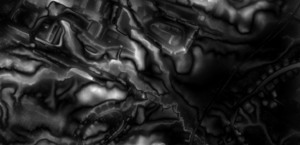
First up is the SFT method.  We will run it now on the LiDAR GeoTIFF.

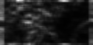
As you can see, when compared to the above original, SFT considers a good part of the image to be unimportant.  There are some areas highlighted, but they do not seem to match up with the features we would be interested in examining.  Next let us try the hill shade TIFF.

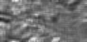
For the hill shade, SFT is a bit all over the place.  It picks up a lot of areas that it thinks should be interesting, but again they do not really match up to the places we would be interested in (house outlines, waterways, etc).

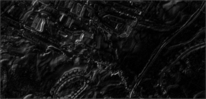
Next we try out the BMS method on the LiDAR GeoTIFF.

You can see that BMS actually did a decent job with the LiDAR image.  Several of the building footprints have edges that are lighter colored and would show up when thresholded / contoured.  The streams are also highlighted in the image.  The roadway and edges at the lower right side of the image are even picked up a bit.

And now BMS run against the hill shade.

The BMS run against the hill shade TIFF is comparable to the run against the LiDAR GeoTIFF.  Edges of the things we would normally be interested in are highlighted in the image.  It does produce smaller highlighted areas on the hill shade versus the original LiDAR.

The obvious downside to these two techniques is that further processing has to be run to produce actual regions of interest.  You would have to threshold the image into a binary image so you could generate contours.  Then you could convert those contours into bounding boxes via other methods.

Object Saliency Method

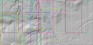
BING is an actual object detector that uses a trained model to find objects in an image.  While not as advanced as many of the modern methods, it does come from 2014 and can be considered the more advanced detection method available for images in OpenCV.  In the config.py file, you can see that with BING, you also have to specify the path to the model that it uses for detection.

Here we see that BING found larger areas of interest than the static salience methods (SFT and BMS).  While the static methods, especially BMS, did a decent job at detecting individual objects, BING generates larger areas that should be examined.  Finally, let us run BING against the hill shade image.

Again we see that BING detected larger areas than the static methods.  The areas are in fact close to what BING found against the LiDAR GeoTIFF.

Results

What can we conclude from all of this?  First off, as usual, LiDAR is hard.  Image processing methods to determine image salience can struggle with LiDAR as many areas of interest are not clearly delineated against the background like they would be in an image of your favorite pet.  LiDAR converted to imagery can be chaotic and really pushes traditional image processing methods to the extremes.

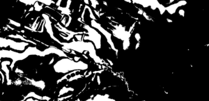
Of all of the OpenCV methods to determine salience, I would argue that BMS is the most interesting and does a good job even on the original LiDAR vs the hill shade TIFF.  If we go ahead and threshold the BMS LiDAR image, we can see that it does a good job of guiding us to areas we would find interesting in the LiDAR data.

The BING objectness model fares the worst against the test image.  The areas it identifies are large parts of the image.  If it were a bigger piece of data, it would basically say the entire image is of interest and not do a great job helping to narrow down where exactly a human would need to look.  And in a way this is to be expected.  Finding objects in LiDAR imagery is a difficult task considering how different the imagery is versus normal photographs that most models are trained on.  LiDAR does not often provide an easy separation of foreground versus background.  High-resolution data makes this even worse as things like a river bank can have many different elevation levels.

Next time we will look at modern deep learning-based methods.  How will they fare?  Will they be similar to the BING objectness model and just tell us to examine large swaths of the image?  Or will they work similarly to BMS and guide us to more individual areas.  We will find out next time.

Stupid LiDAR Tricks Part 1 (Segmentation)

My last few posts have been about applying machine learning to try to extract geographic objects in LiDAR.  I think now I would like to go in another direction and talk about ways to help us find anything in LiDAR.  There is a lot of information in LiDAR, and sometimes it would be nice to have a computer help us to find areas we need to examine.

In this case I’m not necessarily just talking about machine learning.  Instead, I am discussing algorithms that can examine an image and identify areas that have something “interesting” in them.  Basically, trying to perform object detection without necessarily determining the object’s identity.

For the next few posts, I think I’ll talk about:

I have a GitHub repository where I’ll stick code that I’m using for this series.

Selective Search (OpenCV)

This first post will talk about selective search, in this specific case, selective search from OpenCV.  Selective search is a segmentation technique used to identify potential regions in an image that might contain objects. In the context of object detection, it can help to quickly narrow down areas of interest before running more complex algorithms. It performs:

  1. Segmentation of the Image: The first step in selective search is to segment the image into multiple small segments or regions. This is typically done using a graph-based segmentation method. The idea is to group pixels together that have similar attributes such as color, texture, size, and shape.
  2. Hierarchical Grouping: After the initial segmentation, selective search employs a hierarchical grouping strategy to merge these small regions into larger ones. It uses a variety of measures to decide which regions to merge, such as color similarity, texture similarity, size similarity, and shape compatibility between the regions. This process is repeated iteratively, resulting in a hierarchical grouping of regions from small to large.
  3. Generating Region Proposals: From this hierarchy of regions, selective search generates region proposals. These proposals are essentially bounding boxes of areas that might contain objects.
  4. Selecting Between Speed and Quality: Selective search allows for configuration between different modes that trade off between speed and the quality (or thoroughness) of the region proposals. “Fast” mode, for example, might be useful in cases of real-time segmentation in videos.  “Quality” is used when processing speed is less important than accuracy.

Additionally. OpenCV allows you to apply various “strategies” to modify the region merging and proposal process.  These strategies are:

  1. Color Strategy: This strategy uses the similarity in color to merge regions. The color similarity is typically measured using histograms of the regions. Regions with similar colors are more likely to be merged under this strategy. This is useful in images where color is a strong indicator of distinct objects.
  2. Texture Strategy: Texture strategy focuses on the texture of the regions. Textures are usually analyzed using local binary patterns or gradient orientations, and regions with similar texture patterns are merged. This strategy is particularly useful in images where texture provides significant information about the objects, such as in natural scenes.
  3. Size Strategy: The size strategy prioritizes merging smaller regions into bigger ones. The idea is to prevent over-segmentation by reducing the number of very small, likely insignificant regions. This strategy tries to control the sizes of the region proposals, balancing between small regions with no areas of interest to large areas that contain multiple areas of interest.
  4. Fill Strategy: This strategy considers how well a region fits within its bounding box. It merges regions that together can better fill a bounding box, minimizing the amount of empty space. The fill strategy is effective in creating more coherent region proposals, especially for objects that are close to being rectangular or square.

Selective Search in Action

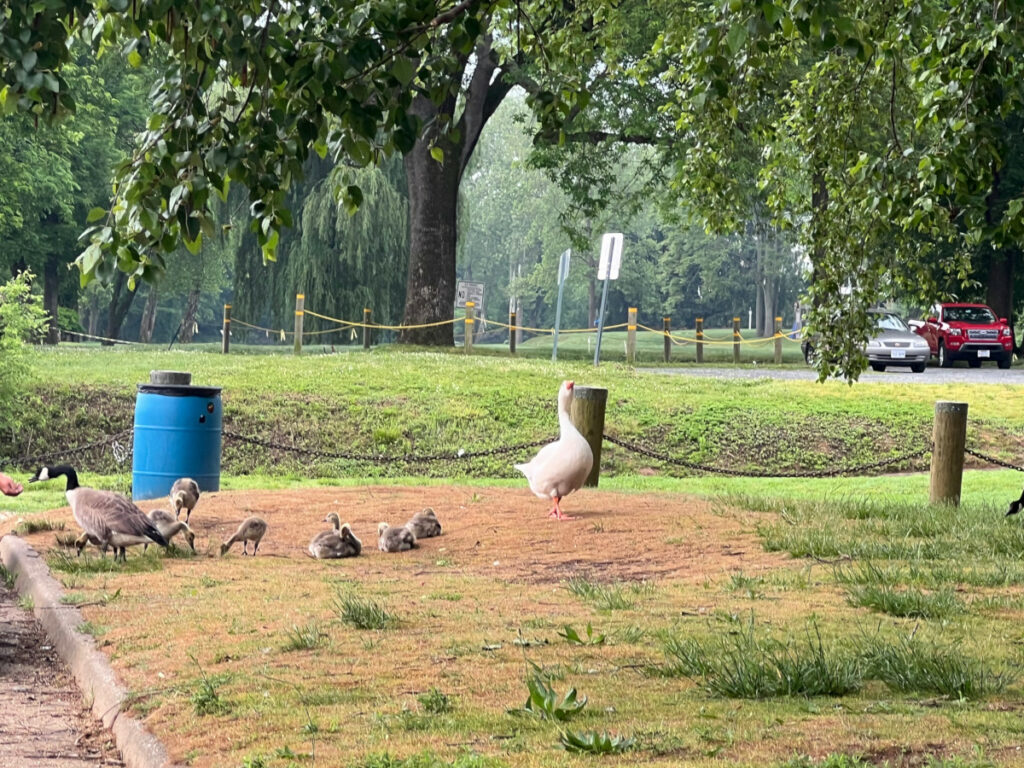
Now let us take a look at how selective search works.  This image is of a local celebrity called Gary the Goose.  To follow along, see the selective_search.py code under the selective_search directory in the above GitHub repository.

Gary the Goose

Now let us see how selective search worked on this image:

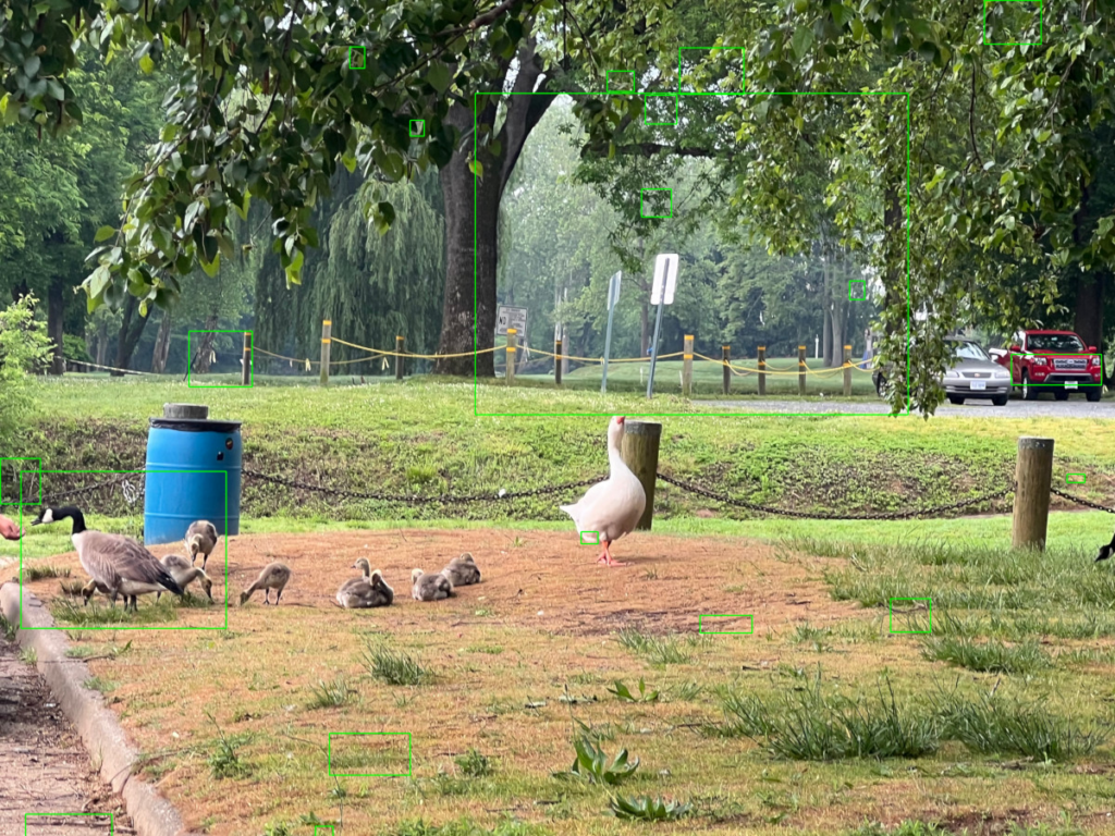
Selective search on image with all strategies applied.

For this run, selective search was set to quality mode and had all of the strategies applied to it.  As you can see, it found some areas of interest.  It got some of the geese, a street sign, and part of a truck.  But it did not get everything, including the star of the picture.  Now let us try it again, but without applying any of the strategies (comment out line 95).

Default selective search with no strategies applied.

Here we see it did about the same.  Got closer to the large white goose, but still seems to not have picked up a lot in the image.

Selective Search on LiDAR

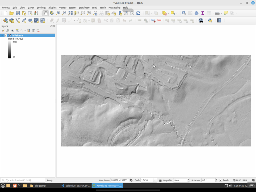
Now let us try it on a small LiDAR segment.  Here is the sample of a townhome neighborhood.

Small LiDAR clip in QGIS

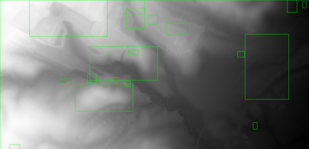
And here is the best result I could get after running selective search:

Selective search run against LiDAR

As you can see, it did “ok”.  It identified a few areas, but did not pick up on the houses or the small creeks that run through the neighborhood. 

Selective Search on a Hill Shade

Can we do better?  Let us first save the same area as a hillshade GeoTIFF.  Here we take the raw image and apply rendering techniques that simulate how light and shadows would interact with the three dimensional surface, making topographic features in the image easier to see.  You can click some of the links to learn more about it.  Here is the same area where I used QGIS to create and export a hill shade image.

LiDAR as a hill shade.

You can see that the hill shade version makes it easier for a human to pick out features versus the original.  It is easier to spot creeks and the flat areas where buildings are.  Now let us see how selective search handles this file.

Selective Search run against a hill shade.

It did somewhat better.  It identified several of the areas where houses are located, but it still missed all of the others.  It also did not pick up on the creeks that run through the area.

Why Did It Not Work So Well?

Now the question you might have is “Why did selective search do so badly in all of the images?”  Well, this type of segmentation is not actually what we would define as object detection today.  It’s more an image processing operation that builds on techniques that have been around for decades that make use of pixel features to identify areas.

Early segmentation methods that led to selective search typically did the following:

  1. Thresholding: Thresholding segments images based on pixel intensity values. This could be a global threshold applied across the entire image or adaptive thresholds that vary over different sized image regions.
  2. Edge Detection: Edge detectors work by identifying boundaries of objects based on discontinuities in pixel intensities, which often correspond to edges.  Some include a pass to try to connect edges to better identify objects.
  3. Region Growing: This method starts with seed points and “grows” regions by appending neighboring pixels that have similar properties, such as color or texture.
  4. Watershed Algorithm: The watershed algorithm treats the image’s intensity values as a topographic surface, where light areas are high and dark areas are low. “Flooding” the surface from the lowest points segments the image into regions separated by watershed lines.

Selective search came about as a hybrid approach that combined computer vision-based segmentation with strategies to group things together.  Some of these were similarity measures such as color, texture, size, and fill to merge regions together iteratively.  It then introduced a hierarchical grouping that built segments at multiple scales to try to better capture objects in an image.

These techniques do still have their uses.  For example, they can quickly find objects on things like conveyor belts in a manufacturing setting, where the object stands out against a uniform background.  However, they tend to fail when an image is “complicated”, like LiDAR as an example or a white goose that does not easily stand out against the background.  And honestly, they are not really made to work with complex images, especially with LiDAR. These use cases require something more complex than traditional segmentation.

This is way longer now than I expected, so I think I will wrap this up here.  Next time I will talk about another computer vision technique to identify areas of an interest in an image, specifically, image saliency.

Applying Deep Learning to LiDAR Part 4: Detection

All of the previous parts of this series have talked about the challenges in training a CNN to detect geological features in LiDAR.  This time I will talk about actually running the CNN against the test area and my thoughts on how it went.

Detection

I was surprised at how small the actual network was.  The xCeption model that I used ended up only being around 84 megabytes.  Admittedly this was only three classes and not a lot of samples, but I had expected it to be larger.

Next, the test image was a 32-bit single band LiDAR GeoTIFF that was around 350 gigabytes.  This might not sound like much, but when you are scanning it for features, believe me it is quite large.

First off, due to the size of the image, and that I had to use a sliding window scan, I knew that the processing time would be long to run detections.  I did some quick tests on subsections and realized that I would have to break up the image and run detection in chunks.  This was before I had put a water cooler on my Tesla P40, and since I wanted to sleep at night, just letting it run to completion was out of the question.  Sleep was not the only concern I had.  I live south of the capital of the world’s last superpower, yet at the time we lost power any time it got windy or rained.  The small chunks meant that if I lost power, I would not lose everything and could just restart it on the interrupted part.

I decided to break the image up into an 8×8 grid.  This provided a size where each tile could be processed in two to three hours.  I also had to generate strips that covered the edges of the tiles to try to capture features that might span two tiles.  I had no idea how small spatially a feature could be, so I picked a 200×200 minimum pixel size for the sliding window algorithm.  This still meant that each tile would have several thousand potential areas to run detections against.  In the end it took several weeks worth of processing to finish up the entire dataset (keeping in mind that I did not run things at night since it would be hard to sleep with a jet engine next to you).

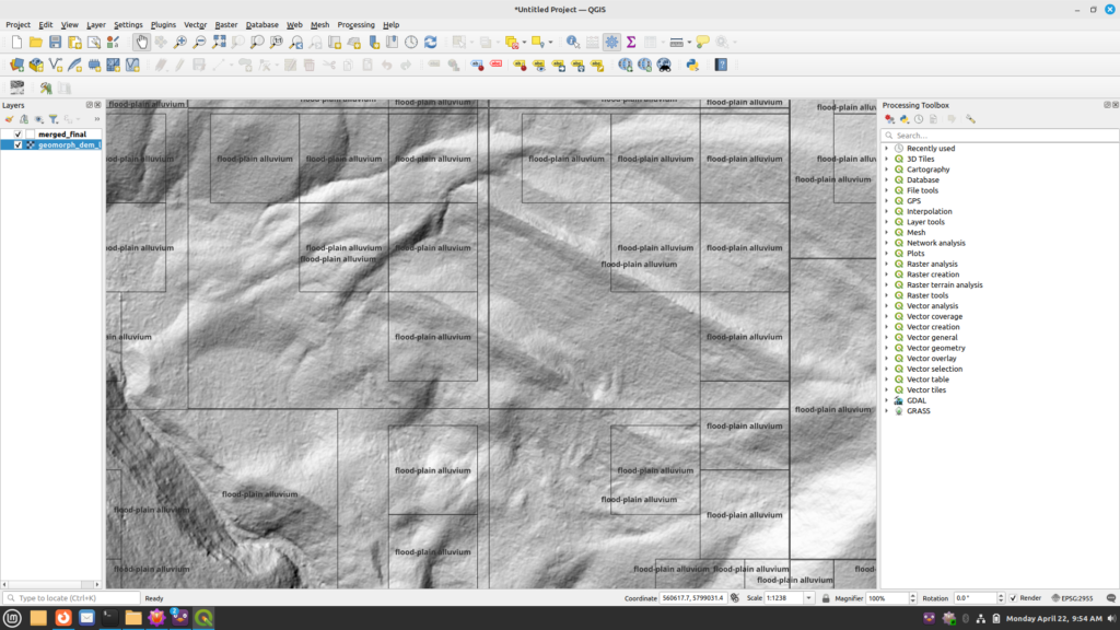
How well did it work?  Well, that’s the interesting part.  I’m not a geomorphologist so I had to rely on the client to examine it.  But here’s an example of how it looks via QGIS:

Sample of LiDAR detections.

As you can see, it tends to see a lot of areas as floodplain alluvium.  After consulting with the subject matter experts, there are a few things that stand out.

  1. The larger areas are not as useful as the smaller ones.  As I had no idea of a useful scale, I did not have any limitations to the size of the bounding areas to check.  However, it appears the smaller boxes actually do follow alluvium patterns.  The output detections need to be filtered to only keep the smaller areas.
  2. It might be possible to run a clustering algorithm against the smaller areas to better come up with larger areas that are correctly in the class.

Closing thoughts and future work

While mostly successful, as I have had time to look back, I think there are different or better ways to approach this problem.

The first is to train on the actual LiDAR points versus a rasterization of them.  Instead of going all the way to rasterization, I think keeping the points that represent ground level as inputs to training might be a better way to go.  This way I could alleviate the issues with computer vision libraries and potentially have a simpler workflow.  I am curious if geographic features might be easier for a neural network to detect if given the raw points versus a converted raster layer.

If I stay with a rasterized version, I think if I did it again I would try one of the YOLO-class models.  These models are state-of-the-art and I think may work better in scanning large areas for smaller scale features as it does its own segmentation and detection.  The only downside to this is I am not entirely sure YOLO’s segmentation would identify areas better than selective search due to the type of input data.

I think it would also be useful to revisit some of the computer vision algorithms.  I believe selective search could be extended to work with higher numbers of bits per sample.  Some of the other related algorithms could likely be extended.  This would help in general with remotely sensed data as it usually contains higher numbers of bits per sample.

While there are a lot of segmentation models out there, I am curious how well any of them would work with this type of data.  Many of them have the same limitations as OpenCV does and cannot handle 32-bits per sample imagery.  These algorithms typically images where objects “stand out” against the background.  LiDAR in this case is much different than the types of sample data that such images were trained on.  For example, here is a sample of OpenCV’s selective search run against a small section of the test data.  The code of course has to convert the data to 8-bits/sample and convert it to a RGB image before running. Note that this was around 300 meg in size and took over an hour to run on my 16 core Ryzen CPU.

You can see that selective search seems to have trouble with this type of LiDAR as there are not anything such as house lots that could be detected. The detections are a bit all over the place.

Well that’s it for now.  I think my next post will be about another thing I’ve been messing with: applying image saliency algorithms to LiDAR just to see if they’d pull anything out.

Applying Deep Learning to LiDAR Part 3: Algorithms

Last time I talked about the problems finding data and in training a machine learning model to classify geologic features from LiDAR.  This time I want to talk about how various libraries can (and cannot) handle 32-bit imagery.  This actually caused most of the technical issues with the project and required multiple work-arounds.

OpenCV and RasterIO

OpenCV is probably the most widely used computer vision library around.  It’s a great library, but it’s written to assume that the entire image can be loaded into memory at once.  To get around this, I had to use the rasterio library as it will read on demand and let you easily read in parts of the image at a time.  To use it with something like Tensorflow, you have to change the data with some code like this:

with rasterio.open(in_file) as src:
    # Read the data as a 3D array (bands, rows, columns)

    # Convert the data type to float32
    data = data.astype(numpy.float32)

    # Transpose the array to match the shape of cv2.imread (rows, columns, bands)
    data = numpy.transpose(data, (1, 2, 0))

    return data
        

Many computer vision algorithms are designed to expect certain types of images, either 8 to 16-bit grayscale or up to 32-bit three channel (such as RGB) images.  OpenCV, one of the most popular, is no different in this aspect .  The mathematical formulas behind these algorithms have certain expectations as well.  Sometimes they can scale to larger numbers of bits, sometimes not.

Finding Areas of Interest

This actually impacts how we search the image for areas of interest.  There are typically two ways to search an image using computer vision: sliding window and selective search.  A sliding window search is a technique used to detect objects or features within an image by moving a window of a fixed size across the image in a systematic manner. Imagine looking through a small square or rectangular frame that you slide over an image, both horizontally and vertically, inspecting every part of the image through this frame. At each position, the content within this window is analyzed to determine whether it contains the object or feature of interest.

Selective Search is an algorithm used in computer vision for efficient object detection. It serves as a preprocessing step that proposes regions in an image that are likely to contain objects. Instead of evaluating every possible location and scale directly through a sliding window, Selective Search intelligently generates a set of region proposals by grouping pixels based on similarity criteria such as color, texture, size, and shape compatibility.

Selective search is more efficient than a sliding window since it returns only “interesting” areas of interest versus a huge number of proposals that a sliding window approach uses.  Selective search in OpenCV is only designed to work with 24 bit images (ie, RGB images with 8 bits per channel).  To use higher-bit data with it, you would have to scale it to 8 bits/channel.  A 32-bit dataset (which includes negative values as these typically indicate no-data areas) can represent 2.15 billion distinct values.  To scale to 8 bits per channel, we would also need to convert it from floating point to 8-bit integer values.  In this case, we can only represent 256 discrete values.  As you can see, this is quite a difference in how many elevations we can differentiate. 

Here’s an example of the areas of interest that a sliding window and image pyramid generates. As you can see, there are a lot of regions of interest that are regularly placed across the image.

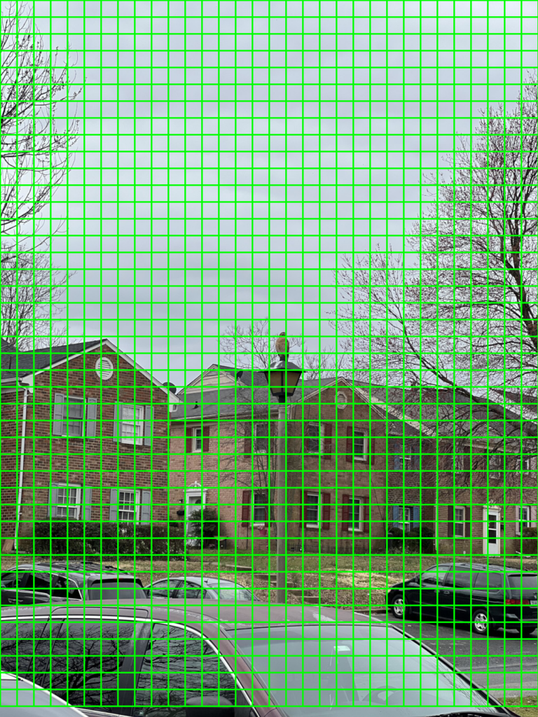
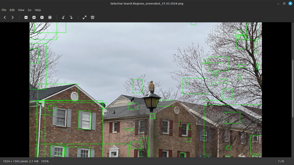
However, selective search is not always perfect.  Below is an example where I ran OpenCV 4’s selective search against an image of mine.  It generated 9,020 proposed areas to search.  I zoomed in to show it did not even show the hawk as a region of interest.

Selective search output run against an image with a hawk.

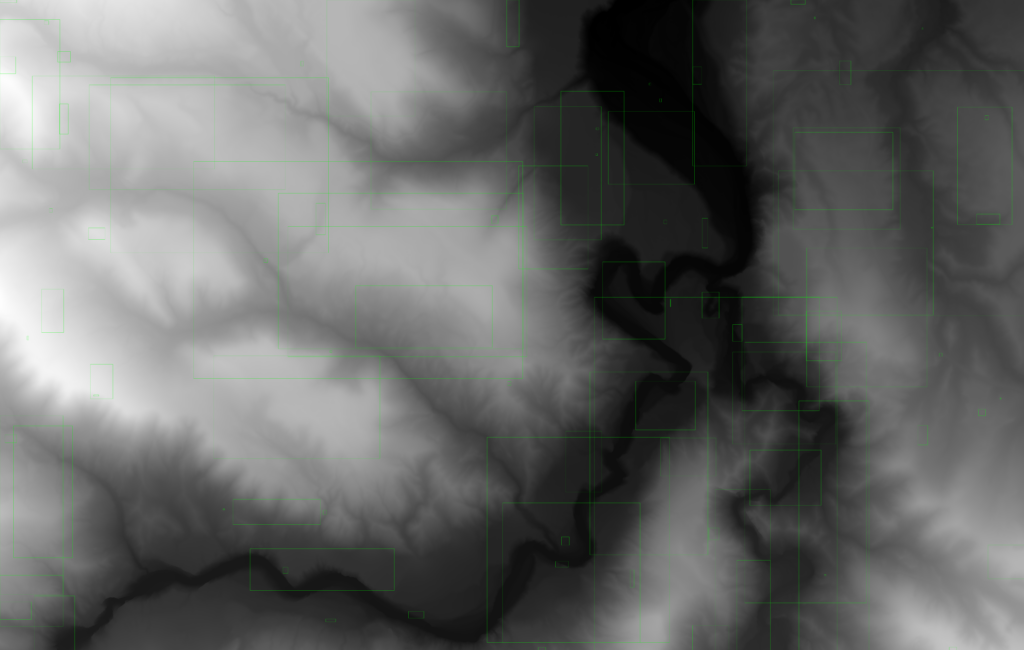
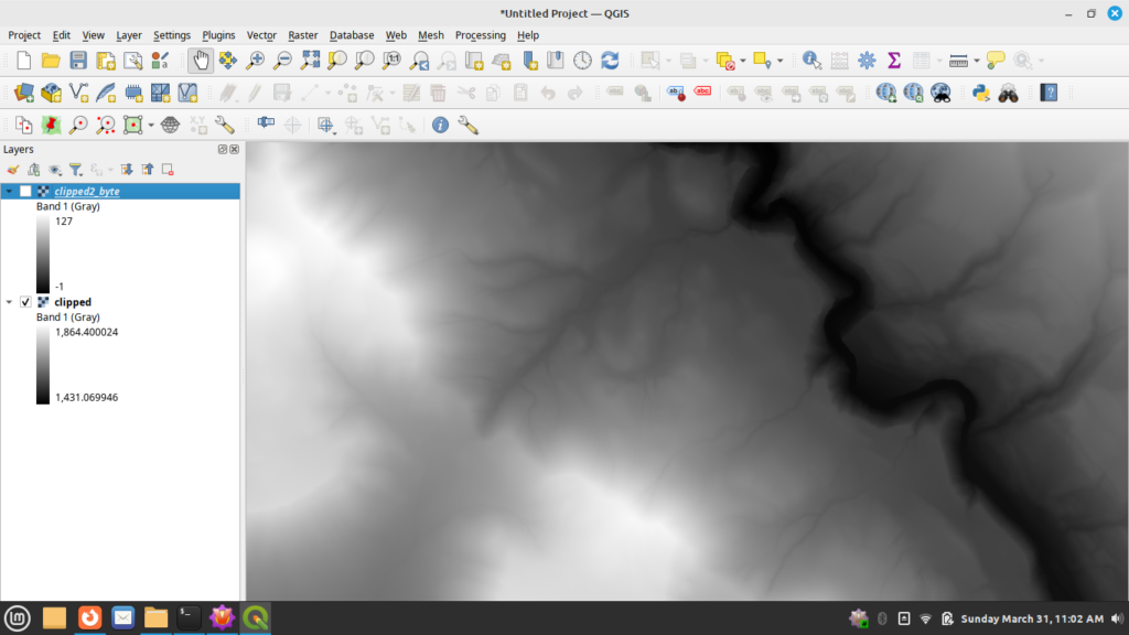
Here’s a clipped version of the input dataset when viewed in QGIS as a 32-bit DEM.  Notice in this case the values range from roughly 1,431 to 1,865.

QGIS with a clip of the original dataset.

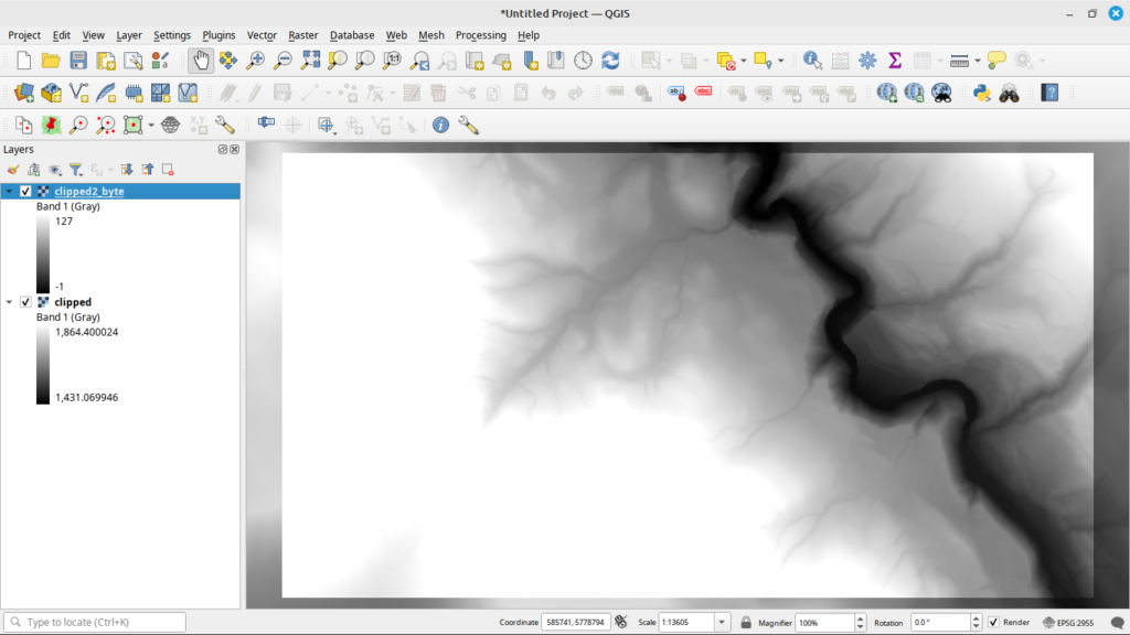
Now here is a version converted to the 8-bit byte format in QGIS.

Same data converted to byte.

As you can see, there is quite a difference between the two files.  And before you ask, int8 just results in a black image no matter how I try to adjust the no-data value.

Tensorflow tf.data Pipeline

So to run this, I set up a Tensorflow tf.data pipeline for processing.  My goal was to be able to turn any of the built-in Tensorflow models into a RCNN.  An interesting artifact of using built-in models, Tensorflow, and OpenCV was that the input data actually had to be converted into RGB format.  Yes, this means a 32-bit grayscale image had to become a 32-bit RGB image, which of course greatly increased the memory requirements.  Here’s a code snippet that shows how to use Rasterio, PIL, and numpy to take an input image and convert it so it’s compatible with the built-in Tensorflow models:

def load_and_preprocess_32bit_image(image_bytes: tensorflow.string) -> numpy.ndarray:
    """Helper function to preprocess 32-bit TIFF image
    Args:
       image_bytes (tensorflow.string): Input image bytes
    Returns:
        numpy.ndarray: decoded image
    """

    with rasterio.io.MemoryFile(image_bytes) as memfile:
        with memfile.open() as dataset:
            image = dataset.read()
    
    image = Image.fromarray(image.squeeze().astype('uint32')).convert('RGB')
    image = numpy.array(image)  # Convert to NumPy array
    image = tensorflow.image.resize(image, local_config.IMAGE_SIZE)

    return image

This function takes the 32-bit DEM, loads it, converts it to a 32-bit RGB image, and then converts it to a format that Tensorflow can work with.  

You can then create a function that can use this as part of a tf.data pipeline by defining a function such as this:


def load_and_preprocess_image_train(image_path, label, in_preprocess_input,
                                    is_32bit=False):
    """ Define a function to load, preprocess, and augment the images
    Args:
        image_path (_type_): Path to the input image
        label (_type_): label of the image
        in_reprocess_input: Function from keras to call to preprocess the input
        is_32bit (bool, optional): Is the image a 32 bit greyscale. Defaults to 
                                   False.

    Returns:
     _type_: Pre-processed image and label
    """

    image = tensorflow.io.read_file(image_path)

    if is_32bit:
        image = tensorflow.numpy_function(load_and_preprocess_32bit_image, 
                                          [image],
                                          tensorflow.float32)
    else:
        image = tensorflow.image.decode_image(image, 
                                              channels=3,
                                              expand_animations=False)
        image = tensorflow.image.resize(image, local_config.IMAGE_SIZE)
     
    image = augment_image_train(image)  # Apply data augmentation for training
    image = in_preprocess_input(image)

    return image, label

Lastly, this can then be set up as a part of your tf.data pipeline by using code like this:

# Create a tf.data.Dataset for training data
train_dataset = tf.data.Dataset.from_tensor_slices((train_image_paths, train_labels))
train_dataset = 
    train_dataset.map(lambda path, label:
        image_utilities.load_and_preprocess_image_train(path,
                                                        label,
                                                        preprocess_input,
                                             is_32bit=local_config.USE_TIF,
                                             num_parallel_calls=tf.data.AUTOTUNE)

(Yeah trying to format code on a page in WordPress doesn’t always work so well)

Note I plan on making all of the code public once I make sure the client is cool with that since I was already working on it before taking on their project.  In the meantime, sorry for being a little bit vague.

Training a Model to be a RCNN

Once you have your pipeline set up, it is time to load the built-in model.  In this case I used Xception from Tensorflow and used the pre-trained model to do transfer learning by the standard omit the top layer, freeze the previous layers, then add a new layer on top that learns from the input.

# Load the model without pre-trained weights
base_model = Xception(weights=local_config.PRETRAINED_MODEL, 
                      include_top=False, 
                      input_shape=local_config.IMAGE_SHAPE,
                      classes=num_classes, input_tensor=input_tensor)

# Freeze the base model layers if we're using a pretrained model

if local_config.PRETRAINED_MODEL is not None:
     for layer in base_model.layers:
         layer.trainable = False

# Add a global average pooling layer
x = base_model.output
x = GlobalAveragePooling2D()(x)

# Create the model
predictions = Dense(num_classes, activation='softmax')(x)
model = Model(inputs=base_model.input, outputs=predictions)

In this case, I used Adam as the optimizer as it performed better than something like the stock SGD and I added in two model callbacks.  The first saves the model to disk every time the validation accuracy goes up, and the second stops processing if the accuracy hasn’t improved over a preset number of epochs.  These are actually built-in to Keras and can be set up as follows:

# construct the callback to save only the *best* model to disk based on 
# the validation loss
model_checkpoint = ModelCheckpoint(args["weights"], 
                                   monitor="val_accuracy", 
                                   mode="max", 
                                   save_best_only=True,
                                   verbose=1)

# Add in an early stopping checkpoint so we don't waste our time
early_stop_checkpoint = EarlyStopping(monitor="val_accuracy",
                                      patience=local_config.EPOCHS_EXIT,
                                      restore_best_weights=True)

You can then add them to a list with

model_callbacks = [model_checkpoint, early_stop_checkpoint]

And then pass that into the model.fit function.

After all of this, it was a matter of running the model.  As you can imagine, training took several hours.  Since this has gotten a bit long, I think I’ll go into how I did the detection stages next time.

Applying Deep Learning and Computer Vision to Lidar Part 2: Training Data

In part one I described some of the issues I had on a recent project that applied deep learning to geographic feature recognition in LiDAR and the file sizes of such data.  This time I want to talk about training data, how important it is, and how little there is for this type of problem.

One of the most important things in deep learning is having both quality training data and a good amount of such data.  I have actually written a previous post about the importance of quality data that you can read here.  At a bare minimum, you should typically have around one thousand samples of each object class you want to train a model to recognize.  Object classes in this case are geographic feature types that we want to recognize.

Training Data Characteristics

These samples should mirror the characteristics of the data that your model will come across during classification tasks.  With LiDAR in GeoTIFF format, the training data should be similar in resolution (0.5 meters in this case) and bit depth (32-bit) to the area for testing.  There should be variability in the training data.  Convolutional neural networks are NOT rotational invariant, meaning that unless you train your model on samples at different angles, it will not automatically recognize features.  In this case, your training LiDAR features should be rotated at different angles to account for differences in projection or north direction.

Balanced Numbers of Features per Class

Your training data should also be balanced, meaning that each class should have roughly the same number of training images where possible.  You can perform some tasks that we will talk about in a bit to help with this, but generally if your model is unbalanced, it could mistakenly “lean” towards one class more than others.

Related to this, when generating your training data, you should make sure your training and testing data contain samples from each of your object classes. Especially when imbalanced, it is very easy to use something like train_test_split from the sklearn library and have it generate a training set that misses some object classes. You should also shuffle your training data so that the samples from each class are sufficiently randomized and the model does not assume that features will appear in a specific order. To alleviate this, make sure you pass in something like:

… = train_test_split(…, shuffle=True, stratify=labels)

where labels is a list of your object classes. For most cases this will ensure the order of your samples is sufficiently randomized and that your training/testing data contains samples of each object class.

Complexity

Geographic features also have a varying complexity in how they appear in LiDAR.  The same feature can “look” differently based on its size or other characteristics.  Humans will always look like humans, so training on them is fairly simple.  Geographic features can be in the same class but appear differently based on factors such as weathering, erosion, vegetation, and even if it’s a riverbed that is dry part of the year.  This increased complexity means that samples need to have enough variability, even in the same object class, for proper training.

Lack of Training Data for This Project

With all of this out of the way, let us now talk about the issues that faced this particular project.  First of all, there is not a lot of labeled training data for these types of features.  At all.  I used various search engines, ChatGPT, even bought a bucket of KFC so I could try to throw some bones to lead me to training data (although I don’t know voodoo so probably read them wrong).

There is a lot of data about these geographic features out there, but not labeled AND in LiDAR format.  There is an abundance of photographs of these features.  There are paper maps of these features.  There are research papers with drawings of these features.  I even found some GIS data that had polygons of these features, but the matching elevation model was too low of a resolution to be useful.

In the end I was only able to find a single dataset that matched the bit depth and spatial resolution that matched the test data.  There were a couple of problems with this dataset though.  First, it only had three feature classes out of a dozen or more.  Second, the number of samples of each of these three classes were way imbalanced.  It broke down like this:

  • Class 1 – 123 samples
  • Class 2 – 2,214 samples
  • Class 3 – 9,700 samples

Realistically we should have just tried for Classes 2 and 3, but decided to try to use various techniques to help with the imbalance.  Plus, since it was a bit of a research project, we felt it would be interesting to see what would happen.

Data Augmentation

There are a few different methods of data augmentation you can do to add more training samples, especially with raster data.  Data augmentation is a technique where you generate new samples from existing data so that you can enhance your model’s generalization and generate more data for training. The key part of this is making sure what the methods you use do not change the object class of the training sample.

Geometric Transformations

The first thing you can do with raster data is to apply geometric transformations (again, as long as they do not change the object class of your training sample).  Randomly rotating your training images can help with the rotational invariance mentioned above.  You can also flip your images, change their scale, and even crop them as long as the feature in the training sample remains.

You can gain several benefits from applying geometric transformations to your training data. If your features can appear at different sizes, scaling transforms can help your model become better generalized on feature size. With LiDAR data, suppose someone did not generate the scene with North at the top. Here, random rotations can help the model generalize to rotation so it can better detect features regardless of angle.

Spatial Relationships

Regardless of what type of augmentations you apply to LiDAR, you have to be mindful that you do not change the spatial characteristics of the data. Consider color space augmentation, something that is common with other areas of deep learning and computer vision. With LiDAR, modifying the brightness/contrast would actually be changing the elevation and/or reflectance values of the data. In some applications, especially those highly based on reflectance values such as detecting types of vegetation, this might be useful. In high-resolution geography, you could end up altering the training data in such a way that it no longer represents real-world features.

Wrapping Up

I think I will end this one here as it got longer than I expected and I’m tired of typing 😉  Next time I’ll cover issues with image processing libraries and 32-bit LiDAR data.

Applying Deep Learning and Computer Vision to LiDAR Part1: File Sizes

Introduction

I recently had an interesting project where a client wanted to see if certain geographic features could be found by using deep learning on LiDAR converted to GeoTIFF format.  I had already been working on some code to allow me to use any of the Tensorflow built-in models as R-CNNs, so this seemed like the perfect opportunity to try this.  This effort wasn’t without issues, and I thought I would detail them here in case anyone else is interested.  File sizes, lack of training data, and a video card with an add-on fan that sounded like a jet engine turned out to be interesting problems for the project.

I decided to split this up into multiple posts.  Here in Part 1, I will be covering the implications of doing deep learning and computer vision on LiDAR where file sizes can range in the hundreds of gigabytes for imagery.

What is LiDAR?

Example LiDAR point cloud courtesy the United States Geological Survey

LiDAR is a technology that uses laser beams to measure distances and movements in an environment. The word LiDAR comes from Light Detection And Ranging, and it works by sending out short pulses of light and measuring the time it takes for them to bounce back from objects or surfaces. You may have even seen it used on your favorite television show, where people will fly a drone to perform a scan of a particular area.  LiDAR can create high-resolution maps of various terrains, such as forests, oceans, or cities. LiDAR is widely used in applications such as surveying, archaeology, geology, forestry, atmospheric physics, and autonomous driving. 

Archaeologists have made a lot of recent discoveries using LiDAR.  In Central and South America, lost temples and other structures from ancient civilizations such as the Aztecs and the Inca have been found in heavily forested areas.  Drone-based LiDAR can be used to find outlines of hard-to-see foundations where old buildings used to stand.

LiDAR scans are typically stored in a point-cloud format, usually LAS or LAZ or other proprietary and unmentionable formats.  These point clouds can be processed in different ways.  It is common to process them to extract the ground level, tree top level, or building outlines.  This is convenient as these points can be processed for different uses, but not so convenient for visualization.

LiDAR converted to a GeoTIFF DEM

These data are commonly converted into GeoTIFF format, a raster file format, so that they can be used in a GIS.  In this form, they are commonly used as high-resolution digital elevation format (DEM) files.  These files can then be used to perform analysis tasks such as terrain modeling, hydrological modeling, and others.

File Sizes

Conversion to GeoTIFF might result in smaller file sizes and can be easier to process in a GIS, but the files can still be very large.  For this project, the LiDAR file was one hundred and three gigabytes. It was stored as a 32-bit grayscale file so that the elevations of each point on the ground could be stored at a high resolution.  This is still an extremely large file, and not able to be fully loaded into memory for deep learning processing unless a very high-end computer was used (spoiler: I do not have a terabyte of RAM on my home computer).

Using CUDA on a GPU became interesting.  I have a 24 gigabyte used Tesla P40 that I got for cheap off eBay.  Deep learning models can require large amounts of memory that can quickly overwhelm a GPU.  Things like data augmentation, where training images are slightly manipulated on the CPU to provide more samples to help with generalization, take up main memory.  The additional size of the 32-bit dataset and training samples led to more memory being taken up than normal.

Deep learning models tend to require training data to be processed in batches.  These batches are small sets of the input data that are processed during one iteration of training.  It’s also more efficient for algorithms such as stochastic gradient descent to work on batches of data instead of the entire dataset during each iteration.  The sheer size of the training data samples meant that each batch took up a large amount of memory.

Finally, it was impossible to run a detection on the entire LiDAR image at one time.  The image had to be broken up into chunks that could be loaded into memory and run in a decent amount of time.  I made a random choice of cutting the image into an 8×8 grid, resulting in sixty-four images.  I wanted to be able to break up the processing so I could run it and combine the results at the end.  At the time, I had not yet water-cooled my Tesla, so the cooling fan I had attached to it sounded like a jet engine while running.  Breaking it into chunks meant that I could process things during the day and then stop at night when I wanted to sleep.  Believe me, working on other projects during the day while listening to that fan probably made me twitch a bit more than normal.

Conclusion

So that’s it for Part 1. I hope I’ve touched on some of the issues that I came across while trying to processing LiDAR with deep learning and computer vision algorithms. In Part 2 I’ll discuss gathering training data (or the lack of available training data).

Image Processing for Beginners: Image Zooming

Today I’m finally going to finish up the series I started on image processing. The goal of this series is to dispel any myths that algorithms that work on images make things up or do strange, arcane magic. The data is there in the images already, and algorithms that work on them simply make things more visible to a human.

My idea for this originally started when people claimed that zooming in on an image using an iPhone was somehow changing it. The claim (politically motivated) was that it changed the semantic content of the image by zooming in or out. So today I’ll wrap up this series by going over how you zoom an image (or make it larger / smaller).  Note this post will be a bit more technical than the last one as I am including code to demonstrate what I am doing.

Semantic content of an image refers to the meaning or information that the image conveys, such as objects, scenes, actions, attributes, etc. For example, if you take a picture of a cat sitting on a table in your kitchen, then the semantic content would be each of the objects that are in that image (cat, table, kitchen).

Images are resized for you automatically all the time, and you are never aware of it mostly.  Your web browser will scale an image so that it fits on your screen.  Mobile devices scale images such that you can fit them on the device display.  You may even have “pinch to zoom” in on an image so you can see things more clearly.  So ask yourself, when you have zoomed in on an image, do new objects suddenly appear in it?  Does an elephant suddenly appear when you zoom in or out of a picture of your children?  You would have noticed this by now should it happen.

Yes, any time you resize an image you do technically change it, as you have to map pixels from the original to the new size.  However, no resizing operation changes the semantic content of the image.  People have been mapping things and rescaling them long before computers have existed.  Architects, draftsmen, cartographers, and others were transforming and resizing things before electricity was discovered.  Just because a computer does it does not mean that suddenly objects get inserted into the image or that the meaning of the image gets changed.

I’ll be using OpenCV 4 and Python 3. For those unaware, OpenCV is an open source computer vision library that has been around for a long time and is used in thousands of projects. The algorithms in it are some of the best around and have been vetted by experts in the field.  The example image I will be using is a public domain image of a fish as can be seen below.

Public Domain Photo of a Fish

To play along at home, I have the source code for this blog post at https://github.com/briangmaddox/blog_opencv_resizing_example

The first thing we do with our sample image is to load it in using OpenCV, print the dimensions, and then display it.

# Load in our input image
input_image = cv2.imread("1330-sole-fish.jpg")

# Get the dimensions of the original image
height, width, channels = input_image.shape

# Print out the dimensions
print(f"Image Width: {width} Height: {height}")

# Display the original image to the user
cv2.imshow("Original Image", input_image)
cv2.waitKey(0)
cv2.destroyAllWindows()

When we run this code, we see our small fish image in a window:

Image of the fish displayed by OpenCV in a window

Next we will do a “dumb” resize of the image.  Here we double each pixel in the X- and Y-directions.  This has the effect of making the image 2x large, effectively zooming in to the image.

empty_mat = numpy.zeros((height * 2, width * 2, channels), dtype=numpy.uint8)

Here empty_mat is an empty image that has been initialized to all zeroes.  Numpy is a well known array library that OpenCV and other packages are built on.  When OpenCV and Python load an image, they store it in what is basically a three dimensional array.  You can think of this as a box where each red, green, and blue channel of the image is contained in the box.

We do the following loop now to copy the pixel to the output empty_mat:

for y in range(height):
    for x in range(width):
        pixel = input_image[y, x]
        empty_mat[y * 2, x * 2] = pixel
        empty_mat[y * 2, x * 2 + 1] = pixel
        empty_mat[y * 2 + 1, x * 2] = pixel
        empty_mat[y * 2 + 1, x * 2 + 1] = pixel

I used a simple loop and assignments to make it easier to see what I am doing.  This loop simply goes through each row of the input image and copies that pixel to four pixels in the output image, effectively doubling the size and zooming the image.

Now we display both the original image and the doubled one.

cv2.imshow("Original Image", input_image)
cv2.imshow("Doubled image", empty_mat)
cv2.waitKey(0)

cv2.destroyAllWindows()
Both the original image and the doubled image displayed by OpenCV

In the above screenshot, we can see that the image has indeed been “zoomed” in and is now twice the size of the original.  Semantically, both images are equal to each other.  You can see the jaggedness of the fish in the doubled image due to the simplistic nature of the resize.  The main take away from this is that it is still the same image, even if it is larger than the original.

Most applications that let you zoom in or resize images use something a bit smarter than a simple doubling of each pixel.  As you can see with the above images, the simple “doubling” results in a jagged image that becomes less visually pleasing as the zoom multiplier gets larger.  This is because to double an image using the simple method, each pixel becomes four pixels.  Four times larger means eight pixels, and so on.  This method also becomes much more complicated if the zoom factor is not an even multiple of two.

Images today are resized using mathematical interpolations.  Wikipedia defines interpolation as “a type of estimation, a method of constructing (finding) new data new points based on the range of a discrete set of known data points.”  “Ah ha!” you might say, this sounds like things are being made up.  And yes they are, but data is not being made up out of the blue.  Instead, interpolations use existing data to mathematically predict data to fill in the gaps. Google, Apple, and other mapping applications use interpolations to fill in the gaps of your position to display on the screen in-between calculating your exact position using the satellites.  Our brains do it when we reach out to catch a fast ball.  Weather and financial forecasters use it every day.

Interpolations have a long history in mathematics.  The Babylonians were using linear and other interpolations as far back as the 300’s BCE to predict the motions of celestial bodies.  As time has gone on, mathematicians have devised better and more accurate methods of predicting values based on existing ones.  Over time, we have gone from the relatively simplistic piecewise constant interpolations to Gaussian processes.  Each advance has made better and closer predictions to what the missing values actually are.

Consider an example using linear interpolation.  This type of problem is often taught in geometry and other math classes.  Assume that we have points on a two-dimensional XY axis such as below.

Plot of the function y=x with the points (2,2) missing.

Here we see we are given a series of (1,1), (3,3), (4,4), (5,5), (6,6), and (7,7).  This is in fact a plot of the function y = x, except I omitted the point (2,2).  We can eyeball and see that the missing y value for x=2 is in fact 2, but let us go through the math.

The formula for linear interpolation is: .  So if we want to solve for the point where x=2, (x1,y1) will be the point (1,1) and (x2, y2) will be the point (3,3).  Plugging these numbers in we get , which indeed gives us y=2 for x=2.  No magic here, just math.

Other types of interpolations, such as cubic, spline, and so on, also have mathematical equations that calculate new values based on existing values.  This point is important to note.  All interpolations use math to calculate new values based on existing ones.  These interpolations have been used over hundreds of years, and are the basis for many things we use today.  No magic, no guessing, no making things up.  I think we can trust them.

So let us get back to image processing.  OpenCV fortunately can use interpolation to resize an image.  As a reminder, we typically do this so that the image is more pleasing to the eye.  Interpolations give us images that are not blocky as in the case of the simple image doubling technique.  First we will use linear interpolation to double the size of the image

double_width = width * 2
double_height = height * 2
linear_double_image = cv2.resize(input_image, (double_width, double_height), interpolation=cv2.INTER_LINEAR)

# Now display both the original and the linear interpolated image to compare.
cv2.imshow("Original Image", input_image)
cv2.imshow("Linear Interpolated image", linear_double_image)
cv2.waitKey(0)
cv2.destroyAllWindows()

To make things explicit, we set new dimensions to twice the width and height of the image and use linear interpolation to scale the image up.

Original image and a linearly interpolated 2x image displayed with OpenCV

Here we see that the interpolated image is not as blocky as the simple pixel doubling image, meaning that yes the new image is a bit different from the original.  However, nothing new has been added to the image.  It has not been distorted and the same semantic content has been preserved.  We can look at what has happened by examining the coordinates at pixel (0,0) in the original image.

Let us take this farther now.  What happens if we increase to four times the original size?

# Linear interpolation to quad size
quad_width = width * 4
quad_height = height * 4

linear_quad_image = cv2.resize(input_image, (quad_width, quad_height), interpolation=cv2.INTER_LINEAR)

# Now display both the original and the linear interpolated image to compare.
cv2.imshow("Original Image", input_image)
cv2.imshow("Linear Interpolated 4x image", linear_quad_image)
cv2.waitKey(0)
cv2.destroyAllWindows()
Original image and a linearly interpolated 4x image displayed by OpenCV

Again, creating a 4x-size image does not introduce any new objects or change the semantic meaning of the image. You may notice that it looks a bit more blurry than the 2x image.  This is because linear interpolation is a simple process. 

Let us see what it looks like using a more rigorous cubic interpolation to create a 4x image.

# Cubic interpolation
cubic_quad_image = cv2.resize(input_image, (quad_width, quad_height), interpolation=cv2.INTER_CUBIC)

# Now display both the original and the linear interpolated image to compare.
cv2.imshow("Original Image", input_image)
cv2.imshow("Cubic Interpolated 4x image", cubic_quad_image)
cv2.waitKey(0)
cv2.destroyAllWindows()
Original image and the cubic interpolated 4x image displayed by OpenCV

We can see that the image does not have as pronounced blockiness that the linearly interpolated image has.  Yes, it is not exactly the same as the original image as we did not simply double each pixel.  However, the semantic contents of the image are the same, even using a different interpolation method.  We did not introduce anything new into the image by resizing it.  The meaning of the image is the same as it was before.  It is just larger so we can see it better.

It is time to wrap this up as it is a longer post than I intended.  You can see from the above that resizing (or zooming in on) an image does not change the content of the image.  We did not turn the fish into a shark by enlarging it.  We did not add another fish to the image by enlarging it.  

I encourage you to try this on your own at home.  Pull out your phone, take a picture, and then zoom in on it.  Your camera likely takes such a high resolution that displaying it on your screen actually reduces some detail, so that you have to zoom in to see the fine detail in the image.  Ask yourself though, is the meaning of the image changed by zooming in or out on it?  Are they still your children, or did zooming in turn them into something else?

I hope that the next time you hear something in the news about image processing, you realize that every algorithm that does this is just math. It is either math to bring out fine details that you cannot normally see in the case of dark images, or math that makes the image larger so that you can better see the smile on a child.  The content of the image is not changed, it is always semantically the same as the original image.