We have finally gotten past the preliminaries, and this series now takes a turn towards what free geospatial data is available and how you can make use of them in free tools. The rest of this series will focus heavily on putting data into a geospatial database, PostGIS in this case. I will also be posting various bash scripts that I have written to make things easier when staging data for import. Many of the datasets are megabytes and gigabytes in size. Trying to use them as a series of files would be slow and very inefficient.

The whole reason people started putting data into geospatial databases is they wanted to use the ability to localize data and use relational query syntax to speed up fetching data. Geospatial databases can physically store data that is spatially near each other in the same locations on disk, commonly called clustering. Spatial indexes can be created that makes it easier for the database to locate information. Combine this with a query that only requests a subset of the data and suddenly you can manipulate large datasets with ease.

“Why would I want to make my own databases when I have Google?” you might ask yourself. You can only get so much out of Google Maps for free. If you make a lot of use of their servers, or if you use it for commercial purposes, you will have to pay. Map data you get back are pre-rendered raster tiles using their styling. Even OpenStreetMap serves up raster tiles already styled. You could use a lot of traffic going back and forth to their servers. If your bandwidth is metered, this could increase your out-of-pocket costs.

If you store the vector data yourself, you have access to the original data that was used to make up the raster tiles from Internet sources. You can do a lot with this type of information, from accurately measuring line segment distances to geolocating street addresses. More importantly, you have access to all the metadata that is in the vector data. You can get more than just a name about a point or area: you can find out who collected that point, when it was collected, and in some cases even who owns a point or area. You can style the data however you want. You can impress all your GIS geek friends. And best of all, you can use it as much as you want without having to pay anyone else.

This post is a bit of a foreshadowing of what is to come. I will provide pointers to the various datasets that will be covered. The idea is that you can read ahead and get a feel for what kinds of information each dataset contains. You might even be amazed at how much is out there.

The first dataset we will cover is the US Census Bureau’s Topologically Integrated Geographic Encoding and Referencing (TIGER) Dataset, which for US citizens is the granddaddy of them all. This dataset has been released since the 1990’s and is one of the original base datasets for OpenStreetMap in the USA. TIGER currently contains a large amount of metadata for each road segment such as left and right street address ranges, what zip codes they are in, and so on.

Next are the data from the OpenStreetMap project. This project was created in 2004 in the UK and has grown to include crowd-sourced data worldwide. It is maintained by volunteers and in many cases is more up to date than many traditional data source. Volunteers can contribute GPS traces or collect data off of aerial photography. In additional to roads, this dataset contains a huge amount of points of interest and trails.

The Natural Earth dataset is a public domain collection that is available at scales of 1:10m, 1:50m, and 1:110m. While not as comprehensive as OpenStreetMap, this dataset contains raster and vector data along with associated metadata. It also contains shaded relief maps that are combined with color-ramped elevation data derived from satellite imagery. It is maintained by the North American Cartographic Information Society (NACIS).

Combined, these three datasets will take up quite a bit of space on your system. You should expect to need at least 30 gigabytes of space on your system, more depending on if you import all of OpenStreetMap or not. We’ll cover that in later installments of this series.

In the meantime, follow the links I’ve posted, play around with tools such as QGIS, and get a feel for how things work.  Hit up the project web pages to learn more about the software and Google for more background if you’re coming into the GIS world fresh.

So in the last installment I mentioned that I would do another article on QGIS.  However, after looking, there is such a large amount of documentation out there that I felt that I would just put links to some good online documents so I would not have to reinvent the wheel.  So here are a few links you can use to learn how to use QGIS as these articles will make use of it later on once I go into how to build your own large holdings of free geospatial data.

• http://www.qgis.org/en/docs/index.html – The QGIS project itself has written up a large amount of very useful documentation on their website.  I would suggest the User’s guide and then the A gentle introduction in GIS.
• http://maps.cga.harvard.edu/qgis/ – This guide is hosted at Harvard University.  While written for 1.7.3, the concepts are the same and gives a thorough howto for QGIS.
• http://qgis.spatialthoughts.com/ – Quantum GIS (QGIS) Tutorials – This site has links on how to do various operations in QGIS.
• http://multimedia.journalism.berkeley.edu/tutorials/qgis-basics-journalists/ – QGIS basics for journalists – Another good howto for using QGIS.

In addition to these, don’t forget to use your favorite search engine to look for QGIS tutorials.  Youtube also has a lot of videos where you can watch, instead of read, how to use QGIS.

Note:

Ok, I admit it.  I did it this way because I’m feeling lazy since I’m sick and figure I would just point to other great tutorials so I can move on to importing data from various sources.

I took a brief vacation so have not updated this in a while. Switched distributions from Fedora KDE Spin back to Kubuntu and had the holidays hit. Then ended up finding out Kubuntu 13.10 did not have the latest QGIS so had to compile the packages for it myself. But now it is time to get back into the swing of things.

We last left off with setting up a geospatial database and putting a small sample Shapefile with a few points so you could get some experience with creating and storing data. However, now that the data is in the database, it would be handy to actually display it instead of just looking at the metadata about it.

Installing QGIS

QGIS is one of the leading open source GIS tools in existence. It can call functions from GRASS to use advanced functionality that is not built-in. It has a Python-based plug-in system with an extensive set of plug ins that perform raster and vector operations in addition to allowing one to use data from Google and Bing as a base map. Put this all together, and you have something that these days can actually take on and surpass the commercial GIS offerings out there.

Installing QGIS is very straight-forward these days. Windows installers can be found at the QGIS website that make use of Cygwin. Most Linux distributions have packages pre-built in their repositories. If you are on Ubuntu, I would recommend that you ignore my previous post on this blog, as the Ubuntu-GIS team has built packages and placed them into the ubuntugis-unstable repository. Do not be fooled by the unstable moniker. I have been using packages from there over the years and have never had any issues with them. Check your distribution repositories and package search tools to find version 2.x for your system.

Using QGIS

Once installed, you will find two different application shortcuts in your Windows/window manager’s menu: QGIS Desktop and QGIS Browser. QGIS Browser is a tool dedicated to making it easy to browse through your geospatial database holdings, be it an ESRI geodatabase or PostGIS. For each layer or data file, you can examine the metadata, preview the file, or examine the attributes stored in the data. The browser was introduced around the QGIS 1.8 time line and is similar to ArcCatalog for the ESRI users in the crowd. The main use for it is to quickly browse and examine your data without having to load it into QGIS proper.

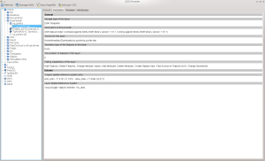
QGIS Browser

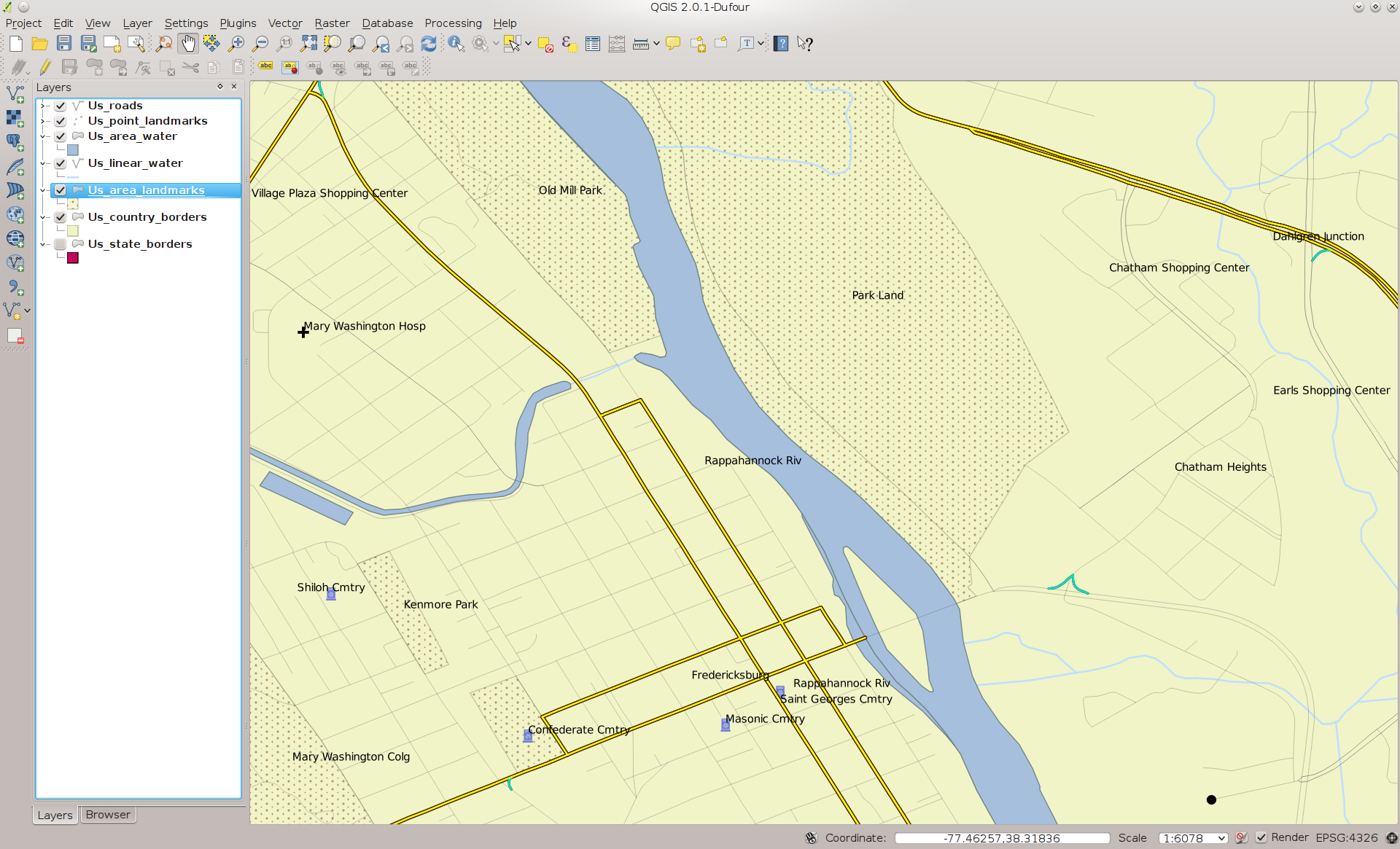
QGIS Desktop is the traditional GIS application that allows you to perform processing on your data in addition to visualizing and examining metadata. The default layout of QGIS is show below.

QGIS Desktop

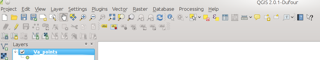
The QGIS 2.x layout differs slightly from the version 1.x layout. By default, along the left side of the window you will find the toolbar containing the add layers buttons for various types of data sources.

QGIS Layers Toolbar

Next to that you will find a tabbed box that displays either the layers window or the browser built-in to QGIS Desktop. The browser here allows you to quickly find data that you can then click and add as a layer into the desktop application.

QGIS Layers and Browser Window

Along the top of the window, you will find the application menus and toolbars for functions such as opening/saving files, zooming, measuring, and other functions. Depending on what plug-ins you have installed an activated, there could be additional menus and toolbars such as the GRASS layers and functions bar.

QGIS Toolbars and Menus

GIS Layers

To use tools such as QGIS, you have to understand how such system work. GISs allow you to manipulate data based on the concept of a layer. Each layer represents a data set, be it raster (think aerial imagery) or vector (think points and lines that represent roads). At a minimum, these data sets are related to each other by their geographic area and temporal parameters. Inside the GIS, you can overlay the different data sets (layers) on top of each other. Usually, you will start with what is called a base map (think of the streets version of Google Maps) and then add more specific data sets on top of that. In the example below (which demonstrates my lack of artistic skills), you can see a Google Roads layer as the base map. Added to that is a river and then a road layer. Inside the GIS, all of these layers would overlay on to the base map so that everything lines up (assuming it has been georeferenced properly).

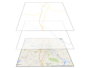
Layers Visualization

Loading Data into QGIS

Now we will use QGIS with a base map and overlay the points that you put into your own geospatial database from the last installment. If you did not put the Shapefile into the geodatabase, you can also simply add it as I will illustrate below.

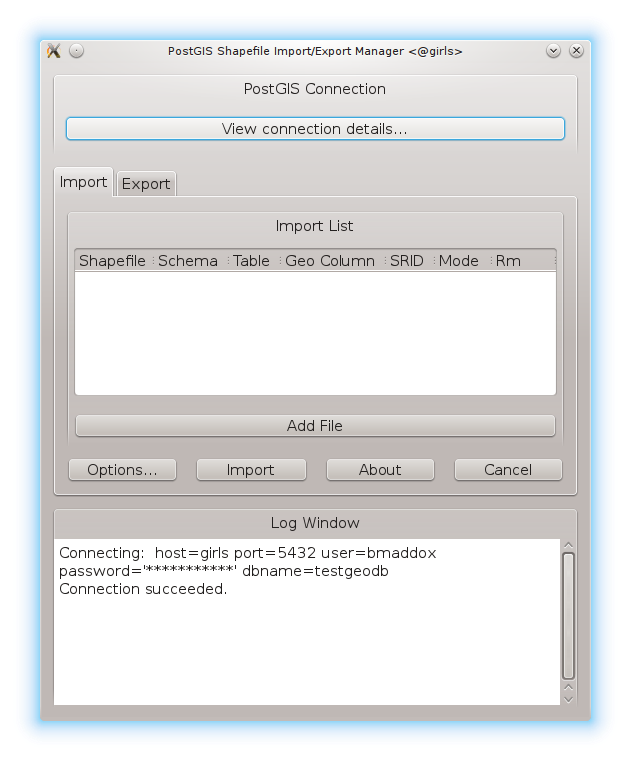
If you set up PostGIS and imported the file into it, start by clicking on the elephant-face icon as shown below.

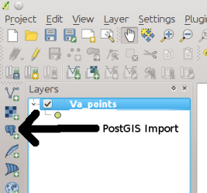
PostGiS Import Button

You will then be presented with the following dialog box.

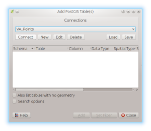
Add PostGIS Table Dialog

Click on the New button and fill out the information similar to the below figure but use your specific host, user, and database names.

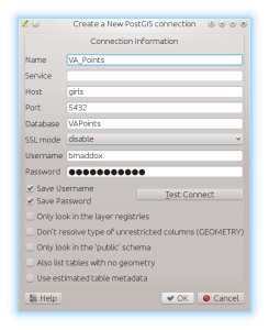
PostGIS Connection Settings

Click OK and then OK again if you chose to save your password like I did. Then, with the VA_Points layer selected in the drop-down, click the Connect button. You should then see an entry under Schema called public. Click on it and you will then see your table name similar to the below figure. Select the points layer and then click the Add button to add this layer to QGIS.

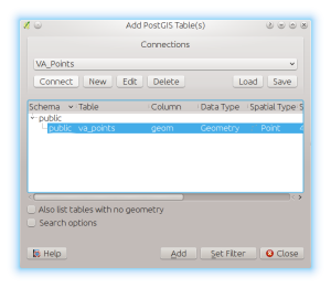
PostGIS Add Layer Dialog

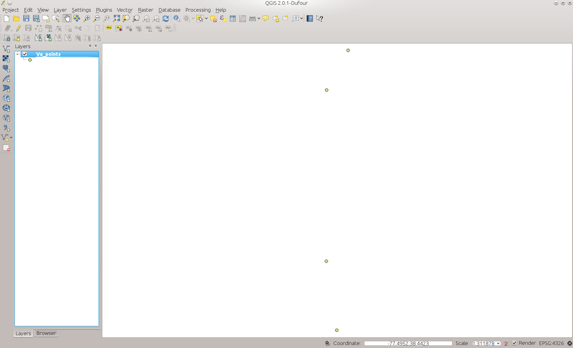
Your QGIS window should look similar to the below. If not, recheck your connection settings and try again.

QGIS after adding the VA_Points layer

Note that if you just download the points layer, click on the Add Vector Layer button which looks similar to a V and is shown below.

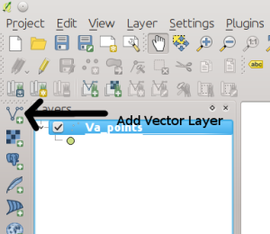
QGIS Add Vector Layer Button

Click the browse button and select the va_points.shp file from the zip archive you downloaded and then click OK. Your screen should look the same as the above.

 Adding a Base Map

Now that we have the points layer added, it is time to add a base map so that you can see how the data overlays.  To do this, we will use the OpenLayers Plugin in QGIS to add a Google Maps satellite image.  First click on the Plugins menu item and select Manage and Install Plugins.  You will see a window similar to this one.

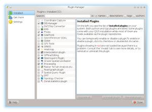
QGIS Plug-in Manager

If you see the OpenLayers Plugin listed in the Installed plug-ins section, click the check box next to it to enable it.  If not, click on Get More tab and type OpenLayers in the Search box.  Click on OpenLayers and then click Install to put it on your system.

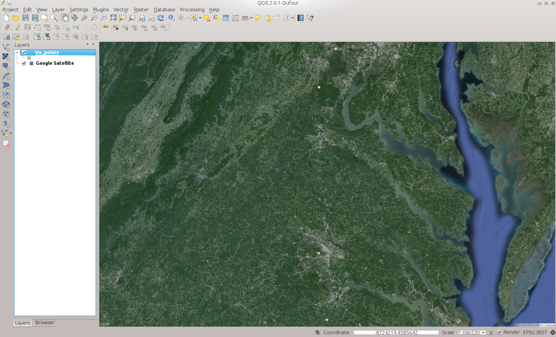
Now that OpenLayers is installed, click on Plugins again, click OpenLayers, and click Add Google Satellite Layer to add it to a new layer in QGIS.

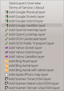
OpenLayers Plug-in Menu

Once done, QGIS will look similar to below.  Do not panic, we will fix it shortly.

QGIS with the Satellite Layer Added

Geographic Extents

I specifically uses this sequence of steps in a work flow to demonstrate another GIS concept – the geographic extent.  Geospatial data has an extent an a time associate with them.  We first loaded the VA Points layer to set the geospatial extent to the area surrounding roughly the middle of Virginia.  The extent on the screen is then based on how much you zoom in or out of the image.  If you zoom in on a point, you are decreasing the geographic area (or extent) that is displayed on the screen.  If you zoom out, you then increase it.

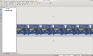
If I had started with just the Google Satellite View, your extent would be as demonstrated in the image.  You then would have had to add the points and then zoom down to where the points are located.  However, as you can see from the above screen shot, when you add a layer using the OpenLayers plugin, it will default to a view such as above.  It appears to be zoomed way out and you see multiple side-by-side images of the Earth.  Plus, it is on top of your image.

Fixing OpenLayers Layers

Fixing this is a very easy task.  First, on the layers side window, notice that the Google Satellite layer is on top of the VA_Points layer.

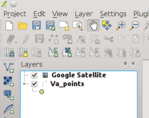
OpenLayers on Top of the Points

Click on the Google Satellite layer and drag it so that it is below the VA_points layer.  Your screen will then look like this.

Satellite Layer Below the Points

Now click on the VA_points layer and select Zoom to Layer Extent.  This will redisplay all of the data so that it fits into the geographic area that the points layer covers.  As you can see below, this also sets the Google Satellite layer to the same extent as the points layer so that the points and satellite layer are both referenced together.

Satellite Layer with the Proper Extent

Changing the Points Color

QGIS will select a random color for your points when you first add the layer.  As you can see from the above screen shot, it choose a green on my system which does not stand out that well over the satellite image.  You can double click on the green dot under the VA_points layer name to change the color.  Double-clicking brings up the properties for the vector layer.  The default should be to display the Style tab.

Vector Style Properties

From here you can change various properties to alter how the layer appears on the screen.  You can select different symbol types, sizes, and other properties for each point.  We will just be changing the color for this example.  Click the color button to bring up the Select Color pop up.  I selected a bright red from the Forty Colors drop-down for the points in this example.

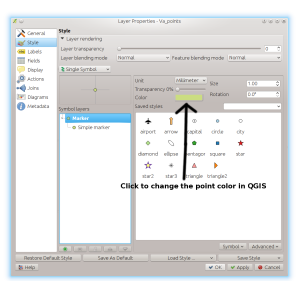
Color Button Location

That’s it.  You now have successfully loaded two different data sets into QGIS.  As homework, find the zoom button in the top menu bar and zoom in to the areas around each point.  You will see that you get more detail from the Satellite layer as you decrease the geographic area around each point.  This is similar to how things would look if you were sitting on your roof looking at the ground versus looking at your house from the International Space Station.

Next Time

Since this post has already gotten very long, next time we will go through some of the other tools that exist inside QGIS, such as viewing metadata for a point and making measurements.

With the release of Ubuntu 13.10, the Ubuntu GIS team has not yet fully rebuilt packages for the new release.  Some have been added, but QGIS has not been updated yet.  Since I did not feel like going back to 1.7.4 after coming back to Kubuntu from the Fedora KDE spin, I decided to build my own debs for 13.10.  After much fighting and patching and hacking I’ve built QGIS 2.0.1 and the necessary related debs that are dependent on what is currently in the ubuntugis-unstable PPA.

To use these, first add the ubuntugis-unstable PPA found at https://launchpad.net/~ubuntugis/+archive/ubuntugis-unstable.  Once you’ve done that, download this 7zip file and decompress it on your system.  I would highly recommend making your own local repository that points to the directory you decompress, but hey it’s your time and effort 😉

Once you are done, do the standard sudo apt-get update, sudo apt-get upgrade, and then sudo apt-get install qgis (assuming you added ubuntugis-unstable and followed my suggestion about making your own local repo).  That should be all you need to do.  I haven’t signed them or anything so you’ll likely need to install from the command line so you can answer yes when prompted about them not being signed.

Since I did this for myself and decided to post the packages until the Ubuntu GIS team has time to build them and put them in their Saucy PPA, I offer no warranty of any type on these.  They work for me.  When the  team does update, use their packages.  I am not affiliated with them in any way, shape, or form (they’d be slumming to hang out with me anyway 😉

• If using them causes your business to fail and you end up homeless on the street, not my fault.
• If using them calls forth Cthulu and he eats your first born, not my fault.
• If you use them to gather coordinates for bombing a military installation and instead hit an orphanage, not my fault.
• If your wife leaves you and you end up writing a Country song named “Feed Jake, Part 2”, not my fault.  However, I’d like to hear it since I have a soft spot for the original.

In this installment, we will look at setting up a geospatial database to store your data. This is not a long post, but the first where you can get your feet wet, so to speak. If you are going to do anything more than just look at a data layer or two, you will want to set up a database. Some vector data sets can be huge (several hundred gigabytes in fact), and opening them in a GIS can take forever. Even if you only want to look at a small part of a file, applications will have to scan through all the data to get to the part you want. Some data sets such as Shapefiles allow you to create index files to help locate the data faster, but you will likely want the added functionality that a spatial database gives you.

The biggest advantage of having a spatial database is that it does a better job of indexing and analyzing the data and stores it for faster access. When your application requests an area, the database will send back only the data covering that area, which will greatly speed up access and processing. Databases can physically sort the data so that features close to each other are stored in the same areas on disk as well.

I am going to describe PostGIS here, mainly because it is the geospatial database I use on a regular basis. Most Linux distributions should have a fairly recent version of the software in their repositories. My Fedora 19 system has version 2.0.3 of PostGIS from the Fedora- and 9.2.5 of PostgreSQL from the updates-testing repositories. Based on your distribution, you should find it in your GUI-based package manager or by running commands such as yum search postgis or apt-cache search postgis from the command line. On Windows, head to http://postgis.net/windows_downloads to find an installer for your platform. You can find install information at http://postgis.net/docs/postgis_installation.html. Again, I am not going to duplicate their instructions here. They spent a lot of time writing it up, so you can read how to install there 🙂  Note that I HIGHLY recommend that you use PostgreSQL 9.1 or later. Version 9.1+ makes it much easier to create a spatial database than previous versions and adds some additional speed benefits.

Depending on how PostGIS was packaged for your system, you might already have a template geospatial database installed. If not, you will want to create one using the instructions found in the postgis_installation link above. Basically, if you are using PostGIS with PostgreSQL 9.1 and above, run the following from a command line:

createdb gis_templatedb
psql -d gis_templatedb -c "CREATE EXTENSION postgis;"
psql -d gis_templatedb -c "CREATE EXTENSION postgis_topology;"

Additionally, if you plan on loading an older database table, run:

psql -d gis_templatedb -f legacy.sql

The above commands create a database and load the geospatial functions from PostGIS into it. These functions allow the database to store spatial data and perform operations such as find all the points nearest to this one and let you search for specific data using SQL operations. The reason you want to have a database template is simple: it makes it much easier to create other geospatial databases. With a template you just have to run a command such as createdb -T my_template_database my_gis_data. Otherwise, you would have to run all of the above commands each time.

Once you have followed the installation instructions from the PostGIS website and have a template in place, you are ready to move on to testing it to make sure everything is OK. Download and unzip this  file somewhere on your system. It is a Shapefile I made of four cities in Virginia. We will use it to test your geospatial database and show you how to load data from it into QGIS.

First, create your geospatial database. Run createdb -T gis_templatedb testgeodb to create your first real geospatial database. If you get any errors, first make sure PostgreSQL is running and then head to the troubleshooting sections of the PostgreSQL website. If it worked correctly, the command will simply return as shown below.

createdb command

PostGIS comes with two versions of a utility to load Shapefile data: shp2pgsql and shp2pgsql-gui. Respectively, the first runs from the command line and you must pass it options to select items such as the EPSG code and the second is a full GUI that lets you click to select your options. As this is a simple Shapefile, we will use the GUI version so you can get some experience loading data.

Find the shp2pgsql-gui command on your system. On Windows it should be under the PostgreSQL menu entry. Under Linux it should be installed to /usr/bin/shp2pgsql-gui. Currently (11/29/2013), if you are running Fedora 19, the PostGIS RPMS contain a broken copy of shp2pgsql and shp2pgsql-gui. You can click here to download fixed RPMS I made that will update PostGIS on your system. The file is a zipfile with the RPMS. Run unzip postgisfixed.zip from a shell to extract the files and then change to the postgisfixed directory. Run rpm -Fvh * as root from the directory to upgrade your copy of PostGIS.

When you run shp2pgsql-gui, it should look like this:

shp2pgsql-gui

The first step is to click the “View connection details” button under the PostGIS Connection label. You will be presented with a window where you can enter in your connection options. Type in your database options and click the OK button. You should see something similar to the below picture showing that your database connection succeeded.

shp2pgsql_dboptions

Now load the Shapefile into shp2pgsql-gui. Click the Add File button and navigate to where you unzipped the va_points.zip file. Click on the va_points.shp file in the sub-directory and shp2pgsql-gui should look similar to the following screen shot.

shp2pgsqlgui_va_points

Before you click the import button, you will likely need to change a few options. Shp2pgsql/shp2pgsql-gui always default to a 0 for the SRID (Spatial Reference system IDentifier). This number specifies the European Petroleum Survey Group (EPSG) code that denotes the coordinate system of the source data. In the case of va_points.shp, double click under SRID and enter in 4326. This code stands for WGS84, which is the projection I used when I created the Shapefile. Once you have done this, click the Import button. Shp2pgsql-gui will pop up a status window and then give you a Shapefile Import Completed message as shown below. That is it, your data should be in your database. If you get any errors, double check the connection parameters and try again. If it still does not work, check the troubleshooting sections on the PostGIS website.

Next time, we will go over installing QGIS so you can look at the data you just imported into your database.

Today there are a huge amount of Open Source geospatial tools out there. The Open Source GIS movement started with libraries to access data formats and has led to full blown geospatial systems today. We’ll look at a few of these that will prove useful to you while you’re working with data. Note that I’m not trying to give an exhaustive explanation how to use the tools here. The projects have already written up a lot of information about how to use them so I’m going to be lazy and not replicate it here. This post will at least give an idea of some of the big players in Open Source GIS so you can continue your investigations there.

Tools

The first project of interest is the Geospatial Data Abstraction Library (GDAL). For developers, GDAL provides a single interface to accessing various raster file formats. For users, it comes with a number of command line utilities that can perform functions from reprojecting data to converting files between various GIS formats. GDAL is used by several other Open Source projects as well for their file format access. We’ll look at some specific uses of GDAL later on. To learn more, visit their website at http://www.gdal.org/.

GDAL comes with several utilities that you might find useful in your geospatial explorations. gdalinfo will give you information about raster GIS files. ogrinfo will provide information on vector file formats. gdaltranslate will convert files to various other formats. gdalwarp will let you convert files to another coordinate system or merge multiple files into a single raster data set.

When appropriate, GDAL provides a wrapper to other libraries to access file formats. libtiff and libgeotiff are used to access the GeoTIFF file format. GeoTIFFs are an extension to the TIFF standard that allows for spatial data to be included with the file. They are mainly used for raster data such as aerial photographs. However, extensions such as 16-bit GeoTIFFs are used to store elevation data where each pixel encodes a height value. LibKML is used to access KML files such as those used with Google Earth. Libpng, libjpeg, and Jasper are used for other formats, and so on.

These libraries also provide useful utilities. One example is listgeo that I used in the last post in this series. Another is tiffinfo that will print out information from standard TIFF tags in a file. tiffcp and geotiffcp will copy files while preserving TIFF and the extended GeoTIFF tags.

As far as full-featured GIS go, the grand-daddy of them all is the Geographic Resources Analysis Support System (GRASS) GIS. GRASS was originally developed from 1982 to 1995 by the US Army Construction Engineering Research Laboratories that is a part of the US Corps of Engineers. For a while it retained its “old school GIS” roots (like early ESRI products) by having everything broken out into programs run from the command line. The Corps ceased developing GRASS around 1995 and it was then taken over by a group of people at Baylor University. It now has gone from simple graphics and requiring a lot of command line experience to a modern GUI thanks to an international group of developers. Of all the Open Source GIS tools, it is the closest competitor to a full featured GIS such as ESRI’s ArcGIS or ERDAS Imagine.

Example of the Modern GRASS GIS GUI

Another powerful Open Source GIS tool is the Quantum GIS (QGIS) project. QGIS started life around 2002 and became a part of the Open Source Geospatial Foundation. It was written using the Qt widget set and features a plugin architecture that allows users to contribute more features using Python or C++. It uses libraries such as GDAL to access numerous raster and vector formats and even includes a plugin so it can act as a front-end to GRASS. Additionally, it can consume OGC web services and interact with Oracle, PostGIS, and ESRI geodatabases. QGIS also features a world-wide group of developers and just recently hit the 2.0 release. For those familiar with ESRI products, it fits in a nebulous area between the old ArcView product and ArcMap. In some ways this author believes it outperforms either product thanks to the plugin architecture and its support of web services. In others it lacks many of the geoprocessing features of the ESRI products. However, it is easily powerful enough for most users who need to work with geospatial data.

QGIS 2.0 Running on Fedora 19

uDig is the third GIS tool in the lineup. It was created by the Canadian company Refractions Research and is based on the Eclipse framework. uDig also features a plugin architecture and can use GRASS for vector processing. Like the others, uDig can ingest OGC web services. Unlike the others, uDig is also used as a base for other GIS applications such as JGrass and Arbonaut. While not necessarily as full featured as QGIS or GRASS, uDig still has its place among the tools.

uDIG screenshot Courtesy Wikipedia

The System for Automated Geospatial Analyses (SAGA) GIS is an Open Source GIS originally developed by the Department of Physical Geography at the University of Gottingen in Germany and now by a group of international volunteers. SAGA also uses GDAL to read a large number of geospatial file formats. It focuses on geoscientific processing and can be called from the R statistical data analysis system. SAGA is similar to QGIS but includes some features not found in that package such as image pattern recognition and more geostatistical functionality. It is still under active development but has not had a new stable release since 2011.

SAGA GIS Screenshot Courtesy Wikipedia

Databases

For storing geospatial data we have two main contenders. Spatial Databases are extensions to traditional relational database systems that allow you to do queries such as “give me all the points within five miles of this location.” The first, PostGIS, is a set of extensions to the PostgreSQL database also developed by Refractions Research and released to the world in 2001. PostGIS is probably the most popular Open Source geospatial database in the world, thanks to its functionality and full implementation of many OGC standards. It started as storing only vector data but was expanded to include raster in version 2.0. It includes geodatabase and geoprocessing functionality not even found in the commercial database offerings. Today it is used by many projects and has support by both proprietary and Open Source GIS tools. Tools such as QGIS can directly communicate with PostGIS to read and write data.

MySQL also has a set of spatial extensions and is catching up to PostGIS in functionality, although it still lags in some areas such as geography and 3D types, SRID projections, and directly querying by a radius. It is not as fully and directly supported by other Open Source GIS tools. However, it is faster for many operations than PostGIS due to the differences in architecture between the two. MySQL Spatial uses a polygon-based model where functions are implemented by bounding polygons.

This is just a brief introduction to Open Source GIS tools out there. I’d highly suggest poking around with your favorite search engine to learn more about what’s available. If you’re an experienced GIS professional, you could get up to speed with QGIS or GRASS fairly quickly. Next time, we’ll start looking at data and how to process it for your needs, including creating spatial databases.