Applying Deep Learning and Computer Vision to Lidar Part 2: Training Data

In part one I described some of the issues I had on a recent project that applied deep learning to geographic feature recognition in LiDAR and the file sizes of such data.  This time I want to talk about training data, how important it is, and how little there is for this type of problem.

One of the most important things in deep learning is having both quality training data and a good amount of such data.  I have actually written a previous post about the importance of quality data that you can read here.  At a bare minimum, you should typically have around one thousand samples of each object class you want to train a model to recognize.  Object classes in this case are geographic feature types that we want to recognize.

Training Data Characteristics

These samples should mirror the characteristics of the data that your model will come across during classification tasks.  With LiDAR in GeoTIFF format, the training data should be similar in resolution (0.5 meters in this case) and bit depth (32-bit) to the area for testing.  There should be variability in the training data.  Convolutional neural networks are NOT rotational invariant, meaning that unless you train your model on samples at different angles, it will not automatically recognize features.  In this case, your training LiDAR features should be rotated at different angles to account for differences in projection or north direction.

Balanced Numbers of Features per Class

Your training data should also be balanced, meaning that each class should have roughly the same number of training images where possible.  You can perform some tasks that we will talk about in a bit to help with this, but generally if your model is unbalanced, it could mistakenly “lean” towards one class more than others.

Related to this, when generating your training data, you should make sure your training and testing data contain samples from each of your object classes. Especially when imbalanced, it is very easy to use something like train_test_split from the sklearn library and have it generate a training set that misses some object classes. You should also shuffle your training data so that the samples from each class are sufficiently randomized and the model does not assume that features will appear in a specific order. To alleviate this, make sure you pass in something like:

… = train_test_split(…, shuffle=True, stratify=labels)

where labels is a list of your object classes. For most cases this will ensure the order of your samples is sufficiently randomized and that your training/testing data contains samples of each object class.

Complexity

Geographic features also have a varying complexity in how they appear in LiDAR.  The same feature can “look” differently based on its size or other characteristics.  Humans will always look like humans, so training on them is fairly simple.  Geographic features can be in the same class but appear differently based on factors such as weathering, erosion, vegetation, and even if it’s a riverbed that is dry part of the year.  This increased complexity means that samples need to have enough variability, even in the same object class, for proper training.

Lack of Training Data for This Project

With all of this out of the way, let us now talk about the issues that faced this particular project.  First of all, there is not a lot of labeled training data for these types of features.  At all.  I used various search engines, ChatGPT, even bought a bucket of KFC so I could try to throw some bones to lead me to training data (although I don’t know voodoo so probably read them wrong).

There is a lot of data about these geographic features out there, but not labeled AND in LiDAR format.  There is an abundance of photographs of these features.  There are paper maps of these features.  There are research papers with drawings of these features.  I even found some GIS data that had polygons of these features, but the matching elevation model was too low of a resolution to be useful.

In the end I was only able to find a single dataset that matched the bit depth and spatial resolution that matched the test data.  There were a couple of problems with this dataset though.  First, it only had three feature classes out of a dozen or more.  Second, the number of samples of each of these three classes were way imbalanced.  It broke down like this:

  • Class 1 – 123 samples
  • Class 2 – 2,214 samples
  • Class 3 – 9,700 samples

Realistically we should have just tried for Classes 2 and 3, but decided to try to use various techniques to help with the imbalance.  Plus, since it was a bit of a research project, we felt it would be interesting to see what would happen.

Data Augmentation

There are a few different methods of data augmentation you can do to add more training samples, especially with raster data.  Data augmentation is a technique where you generate new samples from existing data so that you can enhance your model’s generalization and generate more data for training. The key part of this is making sure what the methods you use do not change the object class of the training sample.

Geometric Transformations

The first thing you can do with raster data is to apply geometric transformations (again, as long as they do not change the object class of your training sample).  Randomly rotating your training images can help with the rotational invariance mentioned above.  You can also flip your images, change their scale, and even crop them as long as the feature in the training sample remains.

You can gain several benefits from applying geometric transformations to your training data. If your features can appear at different sizes, scaling transforms can help your model become better generalized on feature size. With LiDAR data, suppose someone did not generate the scene with North at the top. Here, random rotations can help the model generalize to rotation so it can better detect features regardless of angle.

Spatial Relationships

Regardless of what type of augmentations you apply to LiDAR, you have to be mindful that you do not change the spatial characteristics of the data. Consider color space augmentation, something that is common with other areas of deep learning and computer vision. With LiDAR, modifying the brightness/contrast would actually be changing the elevation and/or reflectance values of the data. In some applications, especially those highly based on reflectance values such as detecting types of vegetation, this might be useful. In high-resolution geography, you could end up altering the training data in such a way that it no longer represents real-world features.

Wrapping Up

I think I will end this one here as it got longer than I expected and I’m tired of typing 😉  Next time I’ll cover issues with image processing libraries and 32-bit LiDAR data.

Applying Deep Learning and Computer Vision to LiDAR Part1: File Sizes

Introduction

I recently had an interesting project where a client wanted to see if certain geographic features could be found by using deep learning on LiDAR converted to GeoTIFF format.  I had already been working on some code to allow me to use any of the Tensorflow built-in models as R-CNNs, so this seemed like the perfect opportunity to try this.  This effort wasn’t without issues, and I thought I would detail them here in case anyone else is interested.  File sizes, lack of training data, and a video card with an add-on fan that sounded like a jet engine turned out to be interesting problems for the project.

I decided to split this up into multiple posts.  Here in Part 1, I will be covering the implications of doing deep learning and computer vision on LiDAR where file sizes can range in the hundreds of gigabytes for imagery.

What is LiDAR?

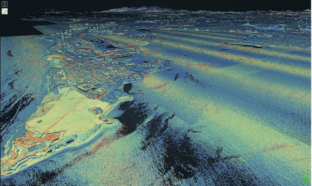
Example LiDAR point cloud courtesy the United States Geological Survey

LiDAR is a technology that uses laser beams to measure distances and movements in an environment. The word LiDAR comes from Light Detection And Ranging, and it works by sending out short pulses of light and measuring the time it takes for them to bounce back from objects or surfaces. You may have even seen it used on your favorite television show, where people will fly a drone to perform a scan of a particular area.  LiDAR can create high-resolution maps of various terrains, such as forests, oceans, or cities. LiDAR is widely used in applications such as surveying, archaeology, geology, forestry, atmospheric physics, and autonomous driving. 

Archaeologists have made a lot of recent discoveries using LiDAR.  In Central and South America, lost temples and other structures from ancient civilizations such as the Aztecs and the Inca have been found in heavily forested areas.  Drone-based LiDAR can be used to find outlines of hard-to-see foundations where old buildings used to stand.

LiDAR scans are typically stored in a point-cloud format, usually LAS or LAZ or other proprietary and unmentionable formats.  These point clouds can be processed in different ways.  It is common to process them to extract the ground level, tree top level, or building outlines.  This is convenient as these points can be processed for different uses, but not so convenient for visualization.

LiDAR converted to a GeoTIFF DEM

These data are commonly converted into GeoTIFF format, a raster file format, so that they can be used in a GIS.  In this form, they are commonly used as high-resolution digital elevation format (DEM) files.  These files can then be used to perform analysis tasks such as terrain modeling, hydrological modeling, and others.

File Sizes

Conversion to GeoTIFF might result in smaller file sizes and can be easier to process in a GIS, but the files can still be very large.  For this project, the LiDAR file was one hundred and three gigabytes. It was stored as a 32-bit grayscale file so that the elevations of each point on the ground could be stored at a high resolution.  This is still an extremely large file, and not able to be fully loaded into memory for deep learning processing unless a very high-end computer was used (spoiler: I do not have a terabyte of RAM on my home computer).

Using CUDA on a GPU became interesting.  I have a 24 gigabyte used Tesla P40 that I got for cheap off eBay.  Deep learning models can require large amounts of memory that can quickly overwhelm a GPU.  Things like data augmentation, where training images are slightly manipulated on the CPU to provide more samples to help with generalization, take up main memory.  The additional size of the 32-bit dataset and training samples led to more memory being taken up than normal.

Deep learning models tend to require training data to be processed in batches.  These batches are small sets of the input data that are processed during one iteration of training.  It’s also more efficient for algorithms such as stochastic gradient descent to work on batches of data instead of the entire dataset during each iteration.  The sheer size of the training data samples meant that each batch took up a large amount of memory.

Finally, it was impossible to run a detection on the entire LiDAR image at one time.  The image had to be broken up into chunks that could be loaded into memory and run in a decent amount of time.  I made a random choice of cutting the image into an 8×8 grid, resulting in sixty-four images.  I wanted to be able to break up the processing so I could run it and combine the results at the end.  At the time, I had not yet water-cooled my Tesla, so the cooling fan I had attached to it sounded like a jet engine while running.  Breaking it into chunks meant that I could process things during the day and then stop at night when I wanted to sleep.  Believe me, working on other projects during the day while listening to that fan probably made me twitch a bit more than normal.

Conclusion

So that’s it for Part 1. I hope I’ve touched on some of the issues that I came across while trying to processing LiDAR with deep learning and computer vision algorithms. In Part 2 I’ll discuss gathering training data (or the lack of available training data).

Image Processing for Beginners: Image Zooming

Today I’m finally going to finish up the series I started on image processing. The goal of this series is to dispel any myths that algorithms that work on images make things up or do strange, arcane magic. The data is there in the images already, and algorithms that work on them simply make things more visible to a human.

My idea for this originally started when people claimed that zooming in on an image using an iPhone was somehow changing it. The claim (politically motivated) was that it changed the semantic content of the image by zooming in or out. So today I’ll wrap up this series by going over how you zoom an image (or make it larger / smaller).  Note this post will be a bit more technical than the last one as I am including code to demonstrate what I am doing.

Semantic content of an image refers to the meaning or information that the image conveys, such as objects, scenes, actions, attributes, etc. For example, if you take a picture of a cat sitting on a table in your kitchen, then the semantic content would be each of the objects that are in that image (cat, table, kitchen).

Images are resized for you automatically all the time, and you are never aware of it mostly.  Your web browser will scale an image so that it fits on your screen.  Mobile devices scale images such that you can fit them on the device display.  You may even have “pinch to zoom” in on an image so you can see things more clearly.  So ask yourself, when you have zoomed in on an image, do new objects suddenly appear in it?  Does an elephant suddenly appear when you zoom in or out of a picture of your children?  You would have noticed this by now should it happen.

Yes, any time you resize an image you do technically change it, as you have to map pixels from the original to the new size.  However, no resizing operation changes the semantic content of the image.  People have been mapping things and rescaling them long before computers have existed.  Architects, draftsmen, cartographers, and others were transforming and resizing things before electricity was discovered.  Just because a computer does it does not mean that suddenly objects get inserted into the image or that the meaning of the image gets changed.

I’ll be using OpenCV 4 and Python 3. For those unaware, OpenCV is an open source computer vision library that has been around for a long time and is used in thousands of projects. The algorithms in it are some of the best around and have been vetted by experts in the field.  The example image I will be using is a public domain image of a fish as can be seen below.

Public Domain Photo of a Fish

To play along at home, I have the source code for this blog post at https://github.com/briangmaddox/blog_opencv_resizing_example

The first thing we do with our sample image is to load it in using OpenCV, print the dimensions, and then display it.

# Load in our input image
input_image = cv2.imread("1330-sole-fish.jpg")

# Get the dimensions of the original image
height, width, channels = input_image.shape

# Print out the dimensions
print(f"Image Width: {width} Height: {height}")

# Display the original image to the user
cv2.imshow("Original Image", input_image)
cv2.waitKey(0)
cv2.destroyAllWindows()

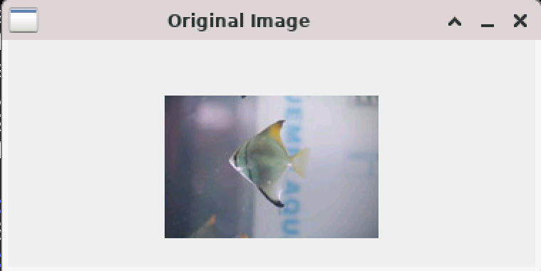
When we run this code, we see our small fish image in a window:

Image of the fish displayed by OpenCV in a window

Next we will do a “dumb” resize of the image.  Here we double each pixel in the X- and Y-directions.  This has the effect of making the image 2x large, effectively zooming in to the image.

empty_mat = numpy.zeros((height * 2, width * 2, channels), dtype=numpy.uint8)

Here empty_mat is an empty image that has been initialized to all zeroes.  Numpy is a well known array library that OpenCV and other packages are built on.  When OpenCV and Python load an image, they store it in what is basically a three dimensional array.  You can think of this as a box where each red, green, and blue channel of the image is contained in the box.

We do the following loop now to copy the pixel to the output empty_mat:

for y in range(height):
    for x in range(width):
        pixel = input_image[y, x]
        empty_mat[y * 2, x * 2] = pixel
        empty_mat[y * 2, x * 2 + 1] = pixel
        empty_mat[y * 2 + 1, x * 2] = pixel
        empty_mat[y * 2 + 1, x * 2 + 1] = pixel

I used a simple loop and assignments to make it easier to see what I am doing.  This loop simply goes through each row of the input image and copies that pixel to four pixels in the output image, effectively doubling the size and zooming the image.

Now we display both the original image and the doubled one.

cv2.imshow("Original Image", input_image)
cv2.imshow("Doubled image", empty_mat)
cv2.waitKey(0)

cv2.destroyAllWindows()
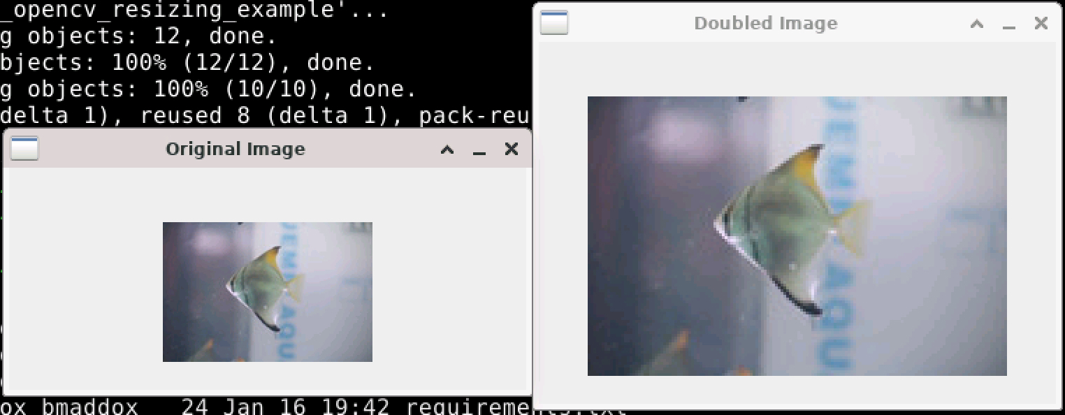
Both the original image and the doubled image displayed by OpenCV

In the above screenshot, we can see that the image has indeed been “zoomed” in and is now twice the size of the original.  Semantically, both images are equal to each other.  You can see the jaggedness of the fish in the doubled image due to the simplistic nature of the resize.  The main take away from this is that it is still the same image, even if it is larger than the original.

Most applications that let you zoom in or resize images use something a bit smarter than a simple doubling of each pixel.  As you can see with the above images, the simple “doubling” results in a jagged image that becomes less visually pleasing as the zoom multiplier gets larger.  This is because to double an image using the simple method, each pixel becomes four pixels.  Four times larger means eight pixels, and so on.  This method also becomes much more complicated if the zoom factor is not an even multiple of two.

Images today are resized using mathematical interpolations.  Wikipedia defines interpolation as “a type of estimation, a method of constructing (finding) new data new points based on the range of a discrete set of known data points.”  “Ah ha!” you might say, this sounds like things are being made up.  And yes they are, but data is not being made up out of the blue.  Instead, interpolations use existing data to mathematically predict data to fill in the gaps. Google, Apple, and other mapping applications use interpolations to fill in the gaps of your position to display on the screen in-between calculating your exact position using the satellites.  Our brains do it when we reach out to catch a fast ball.  Weather and financial forecasters use it every day.

Interpolations have a long history in mathematics.  The Babylonians were using linear and other interpolations as far back as the 300’s BCE to predict the motions of celestial bodies.  As time has gone on, mathematicians have devised better and more accurate methods of predicting values based on existing ones.  Over time, we have gone from the relatively simplistic piecewise constant interpolations to Gaussian processes.  Each advance has made better and closer predictions to what the missing values actually are.

Consider an example using linear interpolation.  This type of problem is often taught in geometry and other math classes.  Assume that we have points on a two-dimensional XY axis such as below.

Plot of the function y=x with the points (2,2) missing.

Here we see we are given a series of (1,1), (3,3), (4,4), (5,5), (6,6), and (7,7).  This is in fact a plot of the function y = x, except I omitted the point (2,2).  We can eyeball and see that the missing y value for x=2 is in fact 2, but let us go through the math.

The formula for linear interpolation is: .  So if we want to solve for the point where x=2, (x1,y1) will be the point (1,1) and (x2, y2) will be the point (3,3).  Plugging these numbers in we get , which indeed gives us y=2 for x=2.  No magic here, just math.

Other types of interpolations, such as cubic, spline, and so on, also have mathematical equations that calculate new values based on existing values.  This point is important to note.  All interpolations use math to calculate new values based on existing ones.  These interpolations have been used over hundreds of years, and are the basis for many things we use today.  No magic, no guessing, no making things up.  I think we can trust them.

So let us get back to image processing.  OpenCV fortunately can use interpolation to resize an image.  As a reminder, we typically do this so that the image is more pleasing to the eye.  Interpolations give us images that are not blocky as in the case of the simple image doubling technique.  First we will use linear interpolation to double the size of the image

double_width = width * 2
double_height = height * 2
linear_double_image = cv2.resize(input_image, (double_width, double_height), interpolation=cv2.INTER_LINEAR)

# Now display both the original and the linear interpolated image to compare.
cv2.imshow("Original Image", input_image)
cv2.imshow("Linear Interpolated image", linear_double_image)
cv2.waitKey(0)
cv2.destroyAllWindows()

To make things explicit, we set new dimensions to twice the width and height of the image and use linear interpolation to scale the image up.

Original image and a linearly interpolated 2x image displayed with OpenCV

Here we see that the interpolated image is not as blocky as the simple pixel doubling image, meaning that yes the new image is a bit different from the original.  However, nothing new has been added to the image.  It has not been distorted and the same semantic content has been preserved.  We can look at what has happened by examining the coordinates at pixel (0,0) in the original image.

Let us take this farther now.  What happens if we increase to four times the original size?

# Linear interpolation to quad size
quad_width = width * 4
quad_height = height * 4

linear_quad_image = cv2.resize(input_image, (quad_width, quad_height), interpolation=cv2.INTER_LINEAR)

# Now display both the original and the linear interpolated image to compare.
cv2.imshow("Original Image", input_image)
cv2.imshow("Linear Interpolated 4x image", linear_quad_image)
cv2.waitKey(0)
cv2.destroyAllWindows()
Original image and a linearly interpolated 4x image displayed by OpenCV

Again, creating a 4x-size image does not introduce any new objects or change the semantic meaning of the image. You may notice that it looks a bit more blurry than the 2x image.  This is because linear interpolation is a simple process. 

Let us see what it looks like using a more rigorous cubic interpolation to create a 4x image.

# Cubic interpolation
cubic_quad_image = cv2.resize(input_image, (quad_width, quad_height), interpolation=cv2.INTER_CUBIC)

# Now display both the original and the linear interpolated image to compare.
cv2.imshow("Original Image", input_image)
cv2.imshow("Cubic Interpolated 4x image", cubic_quad_image)
cv2.waitKey(0)
cv2.destroyAllWindows()
Original image and the cubic interpolated 4x image displayed by OpenCV

We can see that the image does not have as pronounced blockiness that the linearly interpolated image has.  Yes, it is not exactly the same as the original image as we did not simply double each pixel.  However, the semantic contents of the image are the same, even using a different interpolation method.  We did not introduce anything new into the image by resizing it.  The meaning of the image is the same as it was before.  It is just larger so we can see it better.

It is time to wrap this up as it is a longer post than I intended.  You can see from the above that resizing (or zooming in on) an image does not change the content of the image.  We did not turn the fish into a shark by enlarging it.  We did not add another fish to the image by enlarging it.  

I encourage you to try this on your own at home.  Pull out your phone, take a picture, and then zoom in on it.  Your camera likely takes such a high resolution that displaying it on your screen actually reduces some detail, so that you have to zoom in to see the fine detail in the image.  Ask yourself though, is the meaning of the image changed by zooming in or out on it?  Are they still your children, or did zooming in turn them into something else?

I hope that the next time you hear something in the news about image processing, you realize that every algorithm that does this is just math. It is either math to bring out fine details that you cannot normally see in the case of dark images, or math that makes the image larger so that you can better see the smile on a child.  The content of the image is not changed, it is always semantically the same as the original image.

How should we be using ChatGPT?

Large-language model (LLM) systems like ChatGPT are all the rage lately and everyone is racing to figure out how to use them. People are screaming that LLMs are going to put them out of jobs, just like the Luddite movement thought so many years ago.

A big problem is that a lot of people do not understand what things like ChatGPT are and how to use them effectively. Things like ChatGPT rely on statistics. They are trained on huge amounts of text and learn patterns from that text. When you ask them a question, they parse through it and then see what patterns they learned that statistically appear to be the most relevant to your input and then generate output. ChatGPT is a tool that can be effective at helping you to get things done, as long as you keep a few things in mind while using it.

You should already know something about your question before you ask.

Nothing is perfect, and neither are large-language models. You should know something about the problem domain so that you can properly interpret the output you get. LLMs can suffer from what is termed hallucination, where they will blissfully answer your question with incorrect and made-up information. Again, their output is based on statistics, and they’re trained on information that has some inherent biases. They do not understand what you are asking like another human would. You need to check the answer to determine if it is correct.

If you are a software developer, this is especially true when asking ChatGPT to write code for you. There are plenty of examples online of people going back and forth with it until they get working code. My own experience is that it has major issues with the Python bindings for GDAL for some reason.

Be clear with what you ask

ChatGPT uses natural language parsing and deep learning to process your request and then try to generate a response that is statistically relevant. Understand that getting good information out of a LLM can be a back and forth, so the clearer you are, the better it can process what you are asking. Do not ask something like “How do I get rich?” and expect working advice.

Be prepared to break down a complex question into smaller parts

You will not have much luck if you ask something like “Tell me how to replace the headers in my engine” and get complete and specific advise. A LLM does not understand the concept of how to do something like this, so it will not be able to give you a complete step-by-step list (unless some automobile company tries to make a specific LLM). Break down complex questions into smaller parts so that you can combine all the information you get at the end.

Tell it when it is wrong

This is probably mainly important for software developers, but do not be afraid to tell ChatGPT when it is wrong. For example, if you ask it to write some source code for you, and it does not work, go back and tell it what went wrong and what the error was. ChatGPT is conversational, so you may have to have a back and forth with it until it gives you information that is correct.

Ask it for clarification

The conversational nature of ChatGPT means that if you do not understand the response, you can ask it to rephrase things or provide more information. This can be helpful if you ask it about a topic you do not understand. Asking for clarification can also help you to judge whether you are getting correct information.

NEVER GIVE IT PERSONAL INFORMATION

Do NOT, under any circumstances, give ChatGPT personal information such as your social security number, your date of birth, credit card numbers, or any other such information. Interactions with LLMs like ChatGPT are used for further training and for tweaking the information it presents. Understand that anything you ask ChatGPT will permanently become part of its training set, so in theory someone can ask it for your personal information and get it if you provide it.

Takeaways

ChatGPT is a very useful tool, and more and more LLMs are being released on an almost weekly basis. Like any tool, you need to understand it before you use it. Keep in mind that it does not understand what you are asking like a human does. It is using a vast pool of training data, learned patterns, and statistics to generate responses that it thinks you want. Always double check what you get out of it instead of blindingly accepting it.

Some Thoughts on Creating Machine Learning Data Sets

My whole professional career (26 years now!) has been in slinging data around. Be it writing production systems for the government or making deep learning pipelines, I have made a living out of manipulating data. I have always taken pains to make sure what I do is correct and am proud of how obsessive I am about putting things together.

Lately I have been back to doing deep learning and computer vision work and have been looking at some of the open datasets that are out there for satellite imagery. Part of this work has involved trying to combine datasets to train models for object classification from various satellite imagery providers.

One thing I have noticed is that it is still hard to make a good deep learning dataset. We are only human, and we miss things sometimes. It is easy to misclassify things or accidentally include images that might not be a good candidate. Even ImageNet, one of the biggest computer vision and deep learning datasets out there, has been found to contain errors in the training data.

This got me thinking about putting together datasets and what “rules of thumb” I would use for doing so. As there do not seem to be as many articles out there about making datasets versus using them, I thought I would add my two cents on making a good machine learning dataset. This is by no means a criticism about the freely-available datasets out there now. In fact, we should all be thankful so many people are putting them out there, and I hope to add to these soon! So, in no particular order, here we go.

Limit the Number of Object Classes

One thing I have noticed is many datasets try to break out their object classes into too fine of detail. This looks to be especially true for satellite datasets. For example, one popular dataset breaks aircraft down into multiple classes ranging from propeller to trainer to jet aircraft. One problem with this approach is that it becomes easy to pick the wrong category while classifying them. Jet trainers are out there. Should that go into the jet category, or the trainer category? There are commercial propeller aircraft out there. What do we do with them?

It is one thing if you are purposely trying to differentiate different types of aircraft from satellite imagery. Even then, however, I would guess that a neural network would learn mostly the same features for each object class, and you would end up getting the aircraft category correct but have numerous misclassifications for the type. It will also be a lot easier to accidentally mislabel things from imagery while you are building the dataset. Now this is different if you are working with imagery to which only certain types of three letter agencies have access. But, most of us have to make due with the types of imagery that are freely available.

Verify Every Dataset Before Use

We all get into a hurry. We have deadlines, our projects are usually underfunded, and we spend large amounts of time putting out fires. It is still vitally important to not blindly use a dataset to train your model! Consider the below image. In one public domain dataset out there, around eight of these images are all labeled as boats.

Image of a car labeled as a boat.

This is a classical example of “we’re only human.” I would wager that a lot of datasets contain errors such as this. It is not that anyone is trying to purposely mislead you. It just happens sometimes. This is why it is essential to go through your dataset no matter how boring it might be. Labeling is a tough job, and there is probably a room in Hell that tortures people by making them label things all day and night. Again, everyone makes mistakes.

Clean up Your Datasets

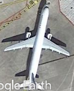
Some datasets out there are derived from Google Earth. It is a source of high quality imagery and for now the terms seem to not require your firstborn or an oath of loyalty. The problem comes when you include things like the image below in your training set.

Here you can see that someone used an aircraft that had the Google Earth watermark superimposed on top of it. If you only have one or two, it likely will not be an issue. However, if you have a lot of things like this, then your network could learn features from the text and start to expect imagery to have this in it. This is an example of where you should practice due diligence in cleaning up your data before putting it into a machine learning dataset.

Avoid Clusters (Unless Looking for Them)

When extracting objects from Google Earth, you might come across something you consider a gold mine. Say you are extracting and labeling cars from imagery, and you come across a full parking lot. This seems like an easy way to suddenly add a lot of training data, and you might end up with a lot of images such as the one below.

In a dataset I recently worked with, there were several object classes that had a lot of images of the same types of objects right next to each other. If you do this, keep in mind that there could be some side effects from having a lot of clusters in your dataset.

  • It could (possibly) be helpful because your object class can present different views if they are present in a cluster. In the above, you can see the top of one bus and the back of another right beside it. This can aid in learning different features for that class.
  • A negative is that if you have a lot of clusters of objects in your training data, your classifier might lean towards detecting objects in groups instead of individual objects. If you are specifically looking for clusters then this is OK. If you want to search for individual ones, then it could hurt your accuracy.
  • The complexity of your training data could increase and lead to slow-downs during the training process by having more features present for each example object than would be present ordinarily.

In general, it is OK to have some clusters of objects in your data. Just be mindful that if you are looking for individual objects, you should try not to have a lot of clusters in your training data.

Avoid Duplicate Objects

This is true for objects in the same class or between object classes. If you have a lot of duplicates, you can run the risk of over-fitting during training. Problems can also arise if you, say, have a car in both a car object class and in a truck class. In this case you can end up with false detections because you accidentally matched the same features in multiple classes.

Pick Representative Training Data

If you are trying to train a model to detect objects from overhead imagery, you would not want to use a training set of pictures people have taken from their cellular phones. Similarly, if you want to predict someone’s mood from a high resolution camera, you would not want to train using fuzzy webcam images. This is stressed in numerous deep learning texts out there, but it is important to repeat. Check if the data you are using for training matches the data you intend to be running your model on. Fitness for use is important.

Invariance

The last thing I want to discuss here is what I feel is one of the most important aspects of deep learning: invariance. Convolutional neural networks are NOT invariant to scale and rotation. They can detect translations, but you do not get scale or rotational invariance by default. You have to provide this using data augmentation during your training phase.

Consider a dataset of numbers that you are using to train a model. This dataset will likely have the numbers written as you would expect them to be: straight up and down. If you train a model on this, it will detect numbers that match a vertical orientation, but accuracy will go down for anything that is off the vertical axis.

Frameworks like Keras make this easy by providing classes or functions that can randomly rotate, shear, or scale images during training before they are input into the network. This helps the classifier learn features in different orientations, something that is important for classifying overhead imagery.

Conclusion

In summary, these are just some general guidelines I use when I am putting together a dataset. I do not always get everything right, and neither will you. Get multiple eyes looking at your dataset and take your time. Labeling is a laborious, and if your attention drifts it is easy to get wrong. The better quality your training data, the better your model will perform.

Finally Upgraded!

If you’ve been trying to come here over the past few days, you might have noticed that this blog has been up and down, changing themes, and what not. I have been having issues upgrading the PHP version on this website and finally got things ironed out thanks to my provider’s awesome support staff! So I promise it should be back to normal now. Mostly. Probably. 😉

Image Processing Basics Part 2

Some Examples

Now that we have some of the basics down, let us look at some practical examples of the differences between how the brain sees things versus how a computer does.

Example image of a clear blue sky

The above photo of a part of the sky was taken by my iPhone 13 Pro Max using the native camera application. There were no filters or anything else applied to it. To our eyes, it looks fairly uniform: mainly blue with some lighter blue towards the right where the sun was the day I took the picture. Each pixel of the image represents the light that hit a sensor in the camera, was processed, and saved.

Our brain does not see a number of individual pixels. Instead, we see large splotches of colors. This is one of the shortcuts our brain does to ease the processing burden. If you look around a room, you do not see individual differences between the colors of the wall. Your wall mainly looks like a uniform color. We simply do not have the processing power to break down the inputs from our eyes into every minute part.

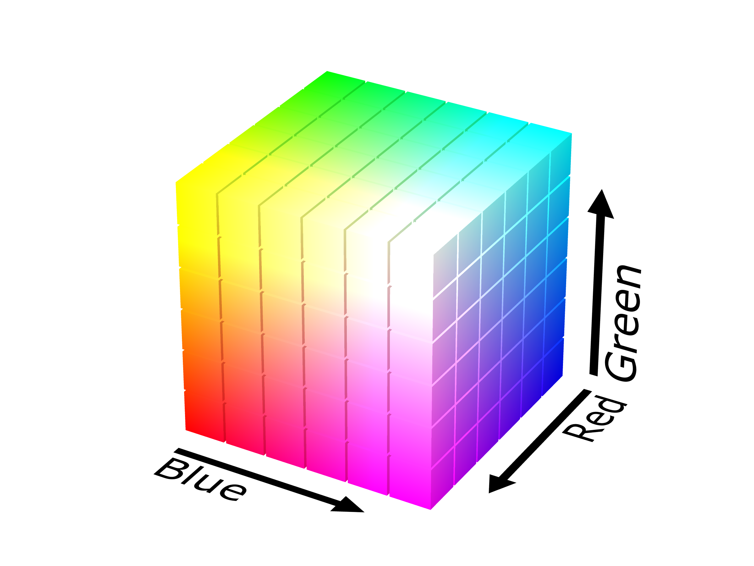
A computer, however, does have the ability to “see” an image in all of its different parts. Computers see everything as a number, be it the 1’s and 0’s of binary or color triplets in the RGB color space. If we look at the RGB color cube below, the computer sees all of the pixels in the above image as clustering somewhere around the lower right side of the cube. See the previous link for more information about the RGB color space.

RGB Color cube from wikipedia
RGB Color Cube (Wikimedia Commons contributors, “File:RGB color solid cube.png,” Wikimedia Commons, https://commons.wikimedia.org/w/index.php?title=File:RGB_color_solid_cube.png&oldid=656872808 (accessed April 18, 2023).

In a computer, the above image is loaded and each pixel is in memory in the form of triplets such as (135, 206, 235), which is the code for a color known as sky blue. The computer also does not have to take any shortcuts when it loads the image, meaning that the representation in memory is exactly the same as the image that was saved from the phone.

If we use the OpenCV library to calculate the histogram of the image and then count the number of colors, we in fact find that there are 2,522 unique colors in the picture of the sky. There is no magic here, we just do not have the same precision that a computer does when it comes to examining images or our environment. The big take away here is this: there is more information encoded in pictures or video than what our brains are capable of perceiving. Just because we cannot see certain details in a image does not mean that they are not there.

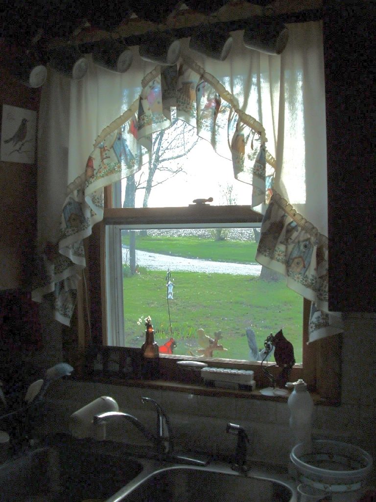
For another example, consider this image below. The edges look like nothing but black, and all you can really see is out of the window. It is definitely underexposed.

Photo out the window of my wife's grandparents' house.
Photo out the window of my wife’s grandparents’ house.

As mentioned above, a computer is able to detect more than our eyes can. Where we just see black around the edges, there is in fact detail there. We can adjust the exposure on the image to brighten it so that our eyes can see these details.

Above image with the exposure and contrast adjusted

With the exposure turned up (and adjusting the contrast as well), we can additionally see a picture of a bird, some dishes, and some cooking implements. This is not magic, nor is it adding anything to the image that was not already there. Image processing like this does not insert things into an image. It only enhances the details of an image so that they are more detectable to the human eye.

Many times, when image processing is in the news, people sometimes assume that it changing an image, or that it is inserting things that were not originally there. When you edit your images on your phone or tablet, you are manipulating the detail that is already in the image. You can enhance the contrast to make the image “pop.” You can change the color tone of the image to make it appear more warm or more cold to your liking. However, this is simply modifying the information that is already in the image to change how it appears to the human eye.

I am making a big deal about this point as future installments in this series will demonstrate how things actually work while hopefully dispelling certain myths that exist in pop culture. I think next time I will cover zooming in or out of an image (aka, resizing). Does it add something into the image or misrepresent it? We will find out.

Image Processing for the Average Person Part 1 – The Human Visual System

There have been a few things in the news about how computers work with images that I feel are a bit misinformed. I believe these reports mislead the average person about how image processing works. As a huge part of my background, and current business, involve image processing, I thought I would start a series of posts about how computers manipulate images, from zooming in and out, to doing enhancement tasks. I hope to give a decent explanation of things so that you, the reader, will have a better understanding and will be able to separate fiction from facts, politics from reality.

First I want to start with the most import part: the human visual system. It is indeed a miracle of evolution, and works pretty well in helping us to navigate our environment. You might be surprised to find, however, that it’s not exactly as good as you might think it is.

Our Vision System Makeup

The Human VisuaL Pathway, Miquel Perello Nieto, CC BY-SA 4.0 https://creativecommons.org/licenses/by-sa/4.0, via Wikimedia Commons

A simplified view of our visual system is that it is made up of the eye, which can be thought of as a camera, the optic nerve (USB cable), and the brain (computer). In reality, there are many more parts to this, including multiple parts of the eye, different parts of the brain that detect and react to different parts of what the eye sees, and so on. There are numerous articles online that break this down into much more detail, but for this series it is enough to use the simplistic point of view.

Physical Characteristics

The specs of our visual system are roughly what is listed below:

  • Much like a physical camera, the performance of our eyes depends a lot on age and the quality of the parts. As we get older, our lens stops performing as well, we get eye floaters, and other issues.
  • Our eyes have receptors in the back that fire when light hits them.
  • Each eye has what is known as a blind spot located where the optic nerve passes through the optic disc. There are no light receptors here so it no data can go to the brain from this area. Do not feel bad, though, as all vertebrate eyes have a blind spot, so it is not just us humans.
  • Our eyes can adapt to a range of intensity of almost ten orders of magnitude. It cannot operate over all of this range simultaneously, however.
  • While we think our eyes see the same all over, we actually only see clearly over the fovea. The fovea is the part of the eye that receives light from the central two degrees of our field of view. To get an idea about how small this is, imagine holding a quarter or half dollar coin at your arm’s length.
  • It is actually hard to assign a resolution such as 1920×1080 to the human eye, as resolutions are dependent on characteristics like sensor size, pixel density, and so on. Instead, we need to think about it in terms of how many pixels make up our vision. Our total field of vision can be thought of as having around 580 megapixels of resolution. Keep in mind that this represents our total field of vision, and that our fovea is the part of the eye that clearly focuses light.
  • Our fovea can be thought of as only being around seven megapixels of resolution. Our eyes are constantly in motion so create our field of view by sending in multiple snapshots to the brain to create our sight. Estimates are that outside of the fovea, the rest of the snapshot is thought to only contain about one megapixel of data.
  • If we want to think in terms of a video frame rate, our eyes and brains can only process around a paltry fifteen frames a second. We see an illusion of motion due to a concept called beta movement. This is chiefly due to how long the visual cortex stores data coming in from the eyes.

Processing Characteristics

Once light coming into our eyes passes to the brain, it runs into several systems that work up to us cognitively recognizing what we are looking at. Again, I am not going to get into the weeds here as there is already plenty of information online about what goes on in portions of the brain such as the visual cortex.

The comparison to a simple camera breaks down here, as our brain has a final say in what we actually see. Parts of the brain work together to help us understand the different parts of the chair, but in the end we decide “Oh I’m looking at a chair.” The brain can also be fooled in its interpretation of what the physical part of the visual system is seeing.

Two profiles or a vase? - Ian Remsen, CC0, via Wikimedia Commons
Two profiles or a vase? – Ian Remsen, CC0, via Wikimedia Commons

An example of this trickery is in optical illusions. This happens when the brain tries to fill in the gaps of information that it needs to decide. It can also misinterpret geometrical properties of an object that results in an incorrect analysis.

The brain merges an amalgamation of what the eyes see into our view of the world. Our eyes are constantly moving, making minute changes to what they are focusing on as we are looking at something. The brain interpolates incoming information to fill in the gaps from parts of the eye like the blind spot and faulty receptors. This means that the brain does a lot of processing to generate what we perceive as our default field of view.

This is a lot of information, so the brain takes as many shortcuts as it can in processing our visual data. We may have a super computer on our necks, but it can only process so much so quickly. This is where comparing our eyes to a camera breaks down as a lot of what we see is based on perception versus physical processing. Our brains cannot store every “megapixel” of what we see in our memories either, so we remember things more as concepts and objects than each individual component of a picture. We simply do not have enough storage to keep everything in our memory.

This finely balanced system of optics and processing and simplification can also break down. We see fast motion as being blurred, or, well, having motion blur. This is because our eyes cannot move fast enough and our brain cannot process fast enough to see individual images, so the brain adds in blur so we understand something is in motion. Now, on a sufficiently high frame rate high definition display, objects are captured without blur, which can mess with our brain’s processing and cause us to have a headache. Think of it as our brain trying to keep up and basically having a blue screen.

This is probably a good place to wrap this up today. I mainly wanted to give a quick explanation of how we see the world to demonstrate that our own eyes are not always perfect, and that a lot goes on behind the scenes to enable our vision.

Next time I’ll start going into some specifics, including showing the difference between what we see and what a computer might see.

When Checkinstall Attacks

The other day I was compiling the latest OpenCV on my computer and had planned on doing what I normally do when it’s done: run checkinstall to build a .deb for it because I like to keep all my files under package management. OpenCV finished compiling fairly quickly (it’s nice when you can do a make -j 16) and I then ran checkinstall.

It crashed while it was running and left a half-installed Debian package of OpenCV on my system. “No problem” I thought, I’ll just uninstall the deb and do a normal make install. Sometimes checkinstall crashes so I didn’t think anything was out of the ordinary. Since I usually put it in /opt/opencv4 it would still be self contained at least.

I noticed a little bit later that my system was acting oddly. Some things wouldn’t run, I couldn’t sudo any more, etc. I rebooted as a first check to see if it was just something random going on. And that’s when my system rebooted to a text mode login prompt. “Huh, maybe the card/drivers didn’t initialize fully I’ll just reboot again.” Nope, no joy still the text login.

I tried to login only to watch the process pause after I typed my password, and then came back up the login prompt. “Odd, maybe I’ll see if it’s something weird and try another virtual console.” Nope, no joy there. Tried to ssh into it, no joy there either. I was worried my SSD was going out. It’s not that old, but still a worry.

So I used my laptop to make a bootable Mint installer and plugged that in and tried to boot. The graphics screen was corrupted and had to use safe mode to log in. “Holy crap, is my graphics card messed up along with the hard drive?” I was worried about this because a new power supply I bought a while back had nuked my old motherboard so had to replace hardware in my system. (That’s a story for another day).

I could still get a GUI when I booted into safe mode from the thumb drive so assumed the open source drivers on the latest Mint installer just didn’t like my card unless I did safe mode.. I did a SMART test to make sure nothing was wrong with the drive. That worked so I ran a fsck to check the integrity of the drive. I then went to set up a chroot to the hard drive so I could run debsums to make sure the packages hadn’t gotten randomly corrupted. And then I noticed a problem.

I couldn’t set up the chroot to work. I kept getting an error about /bin/bash not existing. I checked the /bin directory on the hard drive and sure enough, it was empty save for a broken link to some part of the JDK. “That’s odd, there were no drive errors but /bin is empty.” I thought about things for a moment and it randomly did an ls -ld on the root of the hard drive but didn’t see anything at first.

Then hit it me: “Wait a minute, /bin is supposed to be a link to /usr/bin these days.” I realized that for whatever reason, it looked like checkinstall had replaced the link for /bin with an actual /bin and had randomly placed a link in there for the jdk. I deleted the directory and replaced the link to /usr/bin and rebooted. Boom, system booted normally. Well, mostly normally. CUDA had somehow disappeared from the drive and I had to reinstall it (didn’t use the packages from nVidia since they want to downgrade my video drivers so just did a local install). I ran debsums to check and everything verified properly.

The moral of the story is, it’s good to have debugging skills and know how your computer is supposed to work!